Cosmology · General Relativity

A Statistical Field Theory
for Weak Gravitational Lensing

Automating the diagrammatics of a non-Gaussian driving field

Zheng Zhang
Jodrell Bank Centre for Astrophysics, The University of Manchester

JBCA Meeting · 7 September 2026

sft-wick: A formalism and package for Feynman-diagram expansion and evaluation in stochastic field theories
Z. Zhang · arXiv:2606.19480

Statistical Field Theory for Weak Gravitational Lensing
Z. Zhang, P. Bull, C. Clarkson, A. Nicola · arXiv:2606.19472

background κ-map: Gevolution (ΛCDM relativistic N-body)

The observable

A decade of weak lensing is arriving

Rubin / LSST

~2 bn

Euclid

1.5 bn

Roman

~0.4 bn

Each survey delivers a catalogue of galaxy shapes and fluxes. From it we build two fields on the sky:

\(\kappa\)

convergence, spin-0: images magnified

\(\gamma\)

shear, spin-2: images stretched

Hold on to that split. It comes back as two different pieces of curvature.

spin-2 cosmic shear whisker field: ellipses aligned tangentially in rings around an unseen mass

Coherent distortion around unseen mass.

[Keep this short. It is the hook, not the content.] We are at the start of a remarkable decade. Rubin will image about twenty billion galaxies, a couple of billion of them with shapes good enough for lensing; Euclid one and a half billion with deep infrared; Roman four hundred million, but from space, at a resolution neither of the others can reach. What each survey actually hands you is a catalogue: shapes and fluxes. Out of that catalogue you build two fields. The convergence, kappa, spin-zero, which magnifies images. And the shear, gamma, spin-two, which stretches them, the whiskers on the right. Both are measured, and the paper computes correlation functions of both. Remember that these are two different things, because in a moment they are going to turn out to be driven by two physically different pieces of curvature.

The standard picture

Everything rests on a linear hierarchy

Sum the matter density along the line of sight, weighted by a geometric kernel.

\[ \kappa(\hat{\mathbf n}) = \int_0^{\chi_s}\! d\chi\; W(\chi)\,\delta\!\big(\chi\hat{\mathbf n},\chi\big) \]

Linear in the matter field ⇒ the statistics map one-to-one:

\( \xi_\kappa \leftarrow P_{\rm m}(k) \qquad \zeta_\kappa \leftarrow B_{\rm m}(k_1,k_2,k_3) \)

Two-point in, two-point out. Three-point in, three-point out.

Motivation

But the projection is an approximation

Its known corrections are each bolted on separately, in their own formalisms:

post-Born & lens–lens coupling

beyond-Limber radial mixing

nonlinear growth of the matter field

What does the projection
throw away, and when does it matter?

Ray-tracing combines them, at the price of expensive runs, sample variance, and no clean answer to which mechanism produced a residual.

[Let the question sit. This is what the rest of the talk answers.] It is an approximation, and we know how it fails. The ray bends, so later lenses couple to earlier ones: post-Born. Radial correlations do not collapse to a single shell: beyond-Limber. And the matter field itself grows nonlinearly. The trouble is not that we cannot compute these. It is that each lives in its own formalism, bolted on separately, and they do not naturally compose. To get all of them at once you run a ray-tracing simulation: that works, but it is expensive, it carries sample variance, and when you see a residual it gives you no clean answer about which mechanism produced it. So here is the question I want to answer properly: what does the projection throw away, and when does it matter? To answer it I am going to go back to the geometry.

Part 1 · Back to the geometry

A photon bundle focuses and shears

\[ \dot\theta = -\theta^2-\sigma_+^2-\sigma_\times^2+\textcolor{#9f6209}{\Phi_{00}} \qquad \dot\sigma_{+,\times} = -2\,\theta\,\sigma_{+,\times}+\textcolor{#0f6f96}{\mathcal{W}_{1,2}} \]

Sachs optical scalars and the two curvature sources

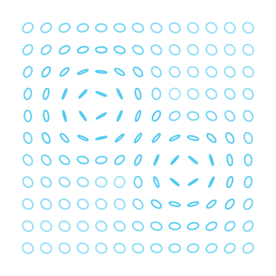
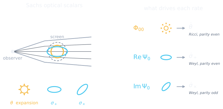
\(\Phi_{00}\) Ricci, the local matter density → drives focusing → \(\kappa\). · \(\Psi_0\) Weyl, the tides from matter off to the side → drives shearing → \(\gamma\).

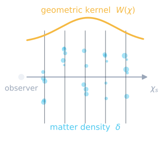
the projection merges these into one \(\kappa\); the Sachs picture keeps them separate, and so does everything that follows

[The spine. Slow down. Point at the two colours.] Forget the projection and follow an actual bundle of light rays through curved spacetime. In general relativity that is the Sachs picture, governed by these optical-scalar equations. A bundle does two things. It changes size, isotropic focusing, the expansion theta. And it changes shape at fixed area, a squeezing, the shear sigma. Now here is the point the projection erases. These are driven by two physically distinct pieces of curvature. Focusing, in amber, is sourced by Ricci curvature, which by Einstein's equations is the local matter density. Shearing, in cyan, is sourced by Weyl curvature, the tidal part, from matter off to the side. And those map onto the two observables from three slides ago: Ricci to convergence, Weyl to shear. Standard lensing merges them into one kappa. We keep them apart, and these two colours run through the rest of the talk.

Part 1 · Reframing

The spacetime is a random field

One realization of the chain the bundle falls through: \(\delta \to \Phi \to \Phi_{00},\,|\Psi_0|\).

Structure formation makes the curvature a draw from an ensemble. So the Sachs system is not an integral to evaluate once. It is a stochastic dynamical system.

\[ \dot{\mathcal X}_a = \underbrace{A_{ab}\mathcal X_b}_{\text{drift}} + \underbrace{\textcolor{#6b34c4}{F_{abc}\mathcal X_b\mathcal X_c}}_{\text{Sachs vertex}} + \underbrace{\textcolor{#9f6209}{\varphi_a}}_{\text{driving field}} \]

\(\mathcal X = (\theta,\sigma_+,\sigma_\times)\) about the background, \(\varphi=(\Phi_{00},\mathcal W_1,\mathcal W_2)\).

Convergence and shear are line-of-sight integrals of that same \(\mathcal X\):

\[ \kappa=-\!\!\int_0^{\lambda}\!\!\mathcal X_1\,d\lambda' , \quad \gamma_+\!\pm i\gamma_\times=-\!\!\int_0^{\lambda}\!\!(\mathcal X_2\pm i\mathcal X_3)\,d\lambda' \]

Two features, and neither is special to lensing:
• quadratic in \(\mathcal X\) • \(\varphi\) is not Gaussian

[Let the field chain sweep for a few seconds before you talk over it.] Here is what the projection hides. The curvature the bundle falls through is not a fixed function. It is one realization of structure in our Universe, built from the matter density through the potential, and that is what is sweeping past on the left. So the Sachs sources are random fields, and the optical scalars are not an integral you evaluate once. They are a stochastic dynamical system. Written out, subtracting the background so there is something linear to expand around, it looks like this. Two things about its shape. It is quadratic in the optical scalars, so the dynamics are nonlinear. And the driving field is the cosmological density and tidal field, which is not Gaussian. Neither is special to lensing, which is why what follows is not either.

Part 1 · Reframing

One trick buys a field theory: the response field

Stochastic ODE

one realization at a time

→

MSR

\(\delta\big[\dot{\mathcal X}-\cdots\big]=\int\!\mathcal D\tilde{\mathcal X}\,e^{i\tilde{\mathcal X}(\cdots)}\)

then marginalise over \(\varphi\)

→

Path integral

\(\langle\mathcal O\rangle=\int\!\mathcal D\mathcal X\,\mathcal D\tilde{\mathcal X}\;\mathcal O\,e^{-S}\)

and the \(S\) in that exponent is, in full:

\[ S[\mathcal X,\tilde{\mathcal X}]\;=\;\underbrace{i\!\int\!\tilde{\mathcal X}_a\big(\dot{\mathcal X}_a-A_{ab}\mathcal X_b\big)}_{\text{linear}}\;-\;i\!\int\!\textcolor{#6b34c4}{F_{abc}\,\tilde{\mathcal X}_a\mathcal X_b\mathcal X_c}\;-\;\textcolor{#9f6209}{W[i\tilde{\mathcal X}]} \]

The same two colours as the equation before: the Sachs vertex and the driving field moved straight into the action.

\[ \textcolor{#9f6209}{W[i\tilde{\mathcal X}]}=\sum_{n\ge2}\frac{i^n}{n!}\int \kappa^{(n)}_{a_1\cdots a_n}\,\tilde{\mathcal X}_{a_1}\!\cdots\tilde{\mathcal X}_{a_n} \]

Marginalising over \(\varphi\) leaves its cumulant generating functional sitting in the action: \(\kappa^{(n)}=\langle\varphi_{a_1}\!\cdots\varphi_{a_n}\rangle_c\). The noise statistics are not bolted on afterwards, and they are the only cosmological input.

[One minute. Do not derive anything.] The construction is Martin, Siggia and Rose. Enforce the equation of motion with a functional delta, Fourier-represent it with an auxiliary field, the response field, then integrate out the driving field. What comes back is the action on the screen. Read it in three pieces. The first is linear: the background focusing, and it is the piece that will give the propagators. The second is the Sachs vertex, in violet, the same term that was quadratic in the equation two slides ago. The third is W, in amber, and it is the driving field's cumulant generating functional: marginalising over the noise does not leave a noise term, it leaves the whole cumulant ladder sitting in the action. So the noise statistics are not bolted on afterwards. They are interaction vertices, and they are the only place cosmology enters. That is the whole reframing. What is left is to expand it, and that is the next slide.

Part 2 · The engine

Split that action, then Wick-contract

Cut it at the Gaussian line: everything quadratic stays, everything else is the perturbation.

\[ \begin{aligned} S_0 &= i\!\int\!\tilde{\mathcal X}_a\big(\dot{\mathcal X}_a-A_{ab}\mathcal X_b\big)-W^{(2)}[i\tilde{\mathcal X}] \\[3pt] S_{\rm int} &= -\,i\!\int\!\textcolor{#6b34c4}{F_{abc}\tilde{\mathcal X}_a\mathcal X_b\mathcal X_c}-\textstyle\sum_{n\ge3}\textcolor{#9f6209}{W^{(n)}[i\tilde{\mathcal X}]} \end{aligned} \]

Every moment then expands about the free theory, and Wick's theorem turns each term into a sum over pairings:

\[ \langle \mathcal O\rangle_S \;=\; \sum_{n}\frac{(-1)^n}{n!}\big\langle\, \mathcal O\, S_{\rm int}^{\,n}\,\big\rangle_{S_0} \]

\(S_0\) is quadratic, so it has exactly two free two-point functions:

\[ \langle \mathcal X_a \mathcal X_b\rangle_{S_0}=\textcolor{#0f6f96}{C_{ab}},\qquad \langle \tilde{\mathcal X}_a \mathcal X_b\rangle_{S_0}=-i\,\textcolor{#9f6209}{R_{ab}} \]

\[ \textcolor{#0f6f96}{C}=\textcolor{#9f6209}{R}\;\kappa^{(2)}\;\textcolor{#9f6209}{R} \]

\(R\) is retarded in \(\lambda\), so it runs outward from us. \(C\) is two of them joined by the drive's two-point function.

\(\langle\tilde{\mathcal X}\tilde{\mathcal X}\rangle_{S_0}=0\): causality kills every response loop.

the response propagator running outward in affine parameter, and the correlation propagator built from two of them

Two propagators and a handful of vertices. The pairings are Feynman diagrams, and these are the symbols on every one that follows.

\(\mathcal V_F\) the Sachs vertex
one, fixed by the geometry

\(\mathcal V_{K_n}\) one per cumulant, \(n\ge3\)
a ladder, and the only cosmological input

[Two beats. Press once in the middle.] Split the action at the Gaussian line. S-nought keeps the linear drift and the second cumulant, which is the Gaussian part of the driving statistics. Everything else is the interaction: the Sachs vertex in violet, and the cumulant ladder from three upwards in amber. Expand any moment about the free theory and you get this sum, and each term is an expectation value in a Gaussian theory, which Wick's theorem factorises into products of two-point functions. [Point right.] S-nought is quadratic, so there are exactly two of those. C, the correlation, and R, the response, which is retarded in affine parameter so it runs outward from us. C is just two R's joined by the drive's two-point function. And the response field has no propagator with itself, which kills every loop. [Press.] Those are the symbols. Two propagators, two vertex families, and Wick's theorem: the pairings are the Feynman diagrams. Nonlinear dynamics and non-Gaussian driving are now in one expansion, in the same currency. That is a bookkeeping problem, and bookkeeping can be automated.

Part 2 · sft-wick

Declare the action, get every diagram

python

from sft_wick import (Field, Vertex,
                      Action, compute_moment)

phi = Field("phi", "physical")
psi = Field("psi", "response")

S = Action([
  Vertex([psi, phi, phi], coupling="F"),
  Vertex([psi, psi, psi], coupling="K",
         local=False),
])

res = compute_moment(
        [phi("x"), phi("y")], S, order=2)

res.draw_diagrams(order=2)

A YAML + CLI layer sits on top:
sft-wick run config.yaml

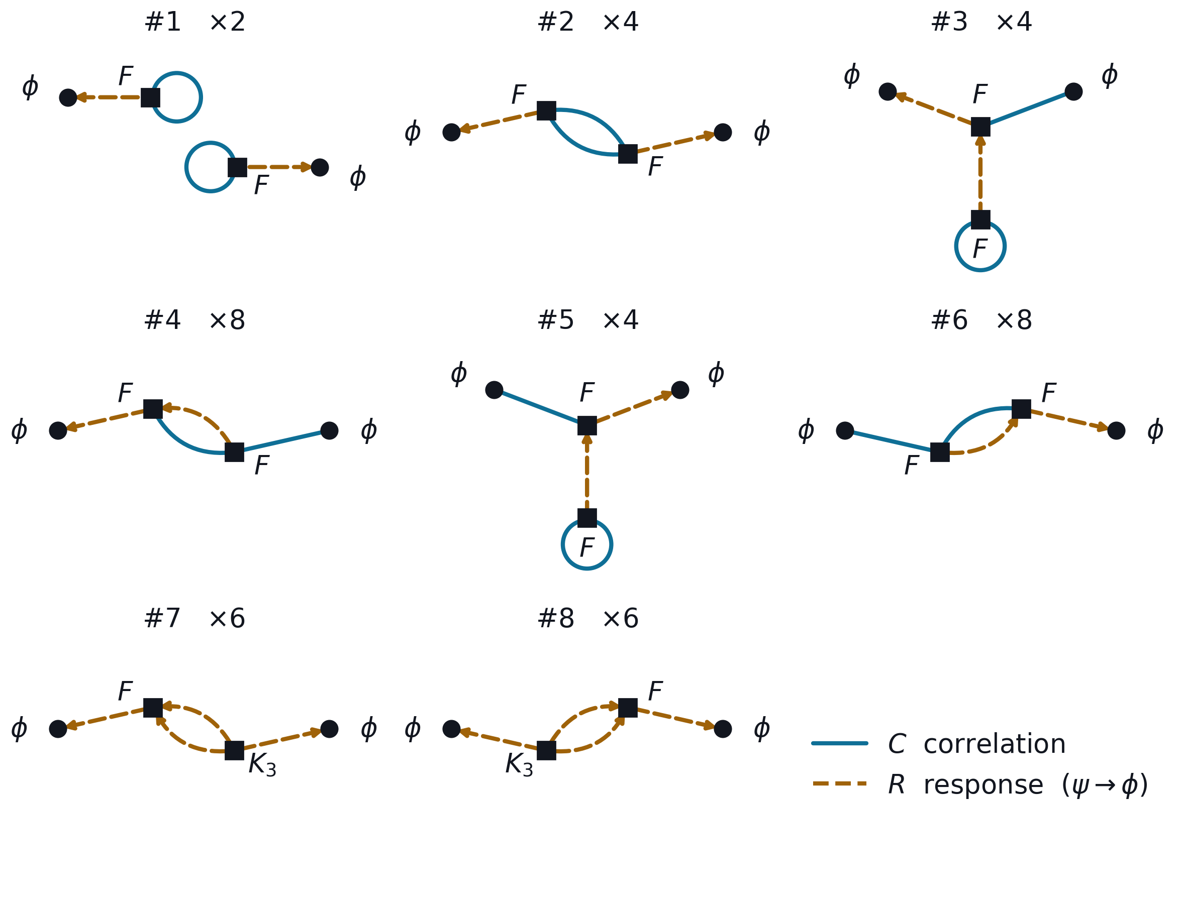
eight order-2 topologies drawn automatically

42 raw Wick pairings collapse to 8 topologies: six with two \(F\) vertices (×2·4·4·8·4·8), two with \(F\,\kappa^{(3)}\) (×6·6) | milliseconds | sft-wick 0.4.2

[Walk the code left to right. Take your time here.] So: sft-wick. On the left is the entire input. A physical field and a response field. Two interactions: the cubic drift vertex, and the three-point cumulant of the noise, which is non-local. You ask for the two-point function to second order, and you ask it to draw. On the right is what comes back, unedited: forty-two Wick pairings collapsed to eight distinct topologies with their multiplicities, drawn automatically, in milliseconds. Six of them have two F vertices. The last two have one F and one cumulant vertex, and notice they carry no cyan line at all, only response legs. Hold on to those two; they are the pair that comes back in the lensing section. Cyan solid is the correlation propagator, amber dashed with the arrow is the response. Squares are vertices, circles are the external operators. Nothing here was drawn by hand. [If asked:] there is a YAML layer on top for people who do not want to write Python at all — you describe the system in a config file and the CLI gives you the diagrams, the numbers and a table.

Part 2 · Does it work?

A system where we can check against the truth

\[ \dot\phi_a = -\gamma\,\phi_a + s\,F_{abc}\,\phi_b\phi_c + \eta_a \]

The same shape as the Sachs system: drift, a quadratic vertex, a random drive. Small enough to integrate directly, so a Langevin simulation gives an independent answer.

For now the noise is Gaussian:

\[ \kappa^{(2)} \propto e^{-|\Delta t|/\sigma_t}\Big(1+\tfrac{|\Delta x|}{\sigma_x}\Big)e^{-|\Delta x|/\sigma_x} \]

\(\kappa^{(n)}=0\) for all \(n\ge3\), so the action has no cumulant vertices.

The drive, the response, and the one-point law it builds. Compare this with the same view under shot noise, three slides on.

two coupled fields on a line · everything in this section is sft-wick's prediction against that simulation

[Half a minute. This is the setup, not a result.] Here is the system. Two coupled fields on a line: linear relaxation, a quadratic self-coupling, a random drive. The same shape as the Sachs system, but small enough to integrate directly, so a brute-force Langevin simulation gives an answer that owes nothing to the diagrammatic expansion. The noise for now is Gaussian. Its second cumulant is the whole story and every higher one is zero, so the action has no cumulant vertices at all. [If anyone asks about the spatial factor: it is what two exponential pulses convolve to. I have chosen it so that when I swap this noise for shot noise in two slides, the second cumulant is identical at every separation and only the higher ones change.] Hold on to that, because it is what the next slide can and cannot test. On the right is the field arriving: the driving noise, the response beneath it, and its one-point law piling up on the Gaussian it is drawn from.

Part 2 · Does it work?

Gaussian baseline: the sum converges to the simulation

Two coupled fields, quadratic drift, Gaussian noise.

orders is enough — the residual sits inside the Monte-Carlo error

But Gaussian noise has no cumulant vertices. This test cannot see the effect we are after.

sft-wick demo 1 · Gauss–Legendre n=20 · 5×10⁴ Langevin realisations · quantitative claims quoted only where the series has saturated

Part 2 · The non-Gaussian demo

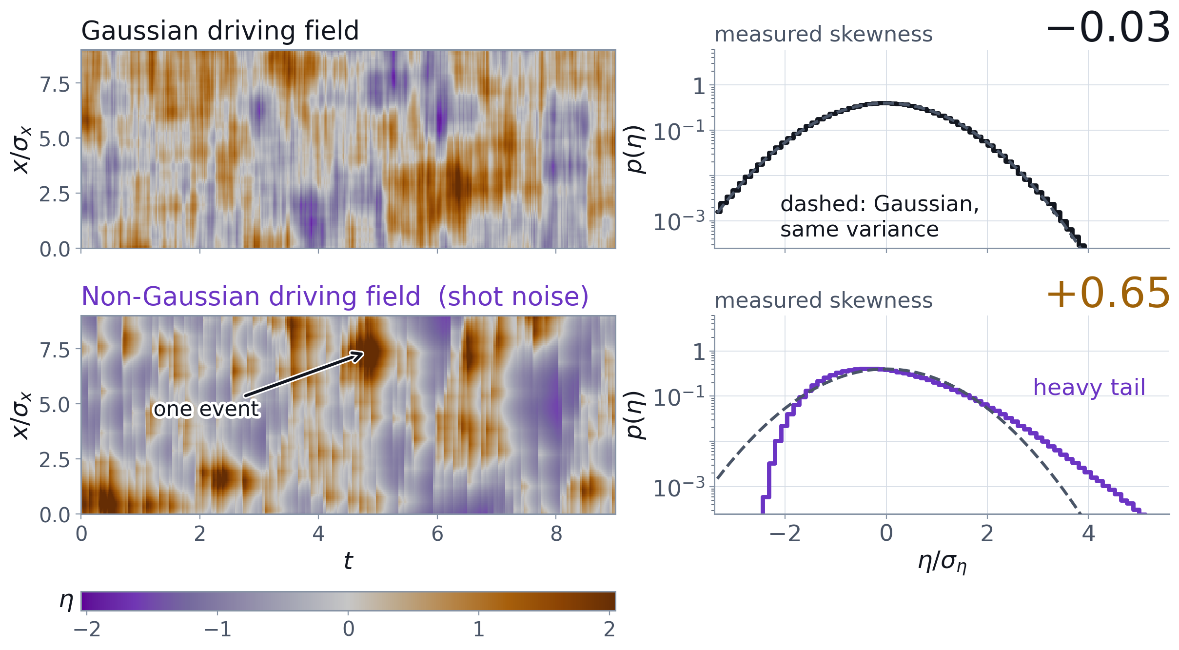
Same power spectrum. Different statistics.

Gaussian driving field versus filtered-Poisson shot noise at matched two-point statistics

\[ \eta(x,t)=\sum_k h\,w(x-x_k)\,g(t-s_k)-\langle\cdot\rangle \qquad n \equiv \nu\,\sigma_t\,\sigma_x = 1 \]

Poisson events at rate \(\nu\), exponential kernels. Same \(\kappa^{(2)}\) as before; now \(\kappa^{(n)}\neq0\) for every \(n\).

\(n\) is events per correlation volume · measured on these two realisations: two-point functions matched to ~2%, skewness −0.03 vs +0.65, excess kurtosis +0.01 vs +0.50 · Campbell's theorem gives every cumulant in closed form

[Point at the two rows.] This is what makes the test sharp. The top row is Gaussian noise. The bottom row is a filtered Poisson process — discrete events arriving at random in space and time, each one kicking the field with an exponential profile. The two are matched at second order: same variance, same correlation length, to a couple of per cent in these realisations. If you only measured the power spectrum you would struggle to tell them apart. Where they differ is unambiguous — skewness minus nought point nought three against plus nought point six five, and you can see it: the bottom row arrives in lumps. And the reason to choose this model is Campbell's theorem — every cumulant of a filtered Poisson process is known analytically, to all orders. So I have a non-Gaussian driving field where I know the exact answer.

Part 2 · the non-Gaussian demo

Same variance throughout. The distribution is not the dashed curve.

Part 2 · Non-Gaussian demo · the exact tier

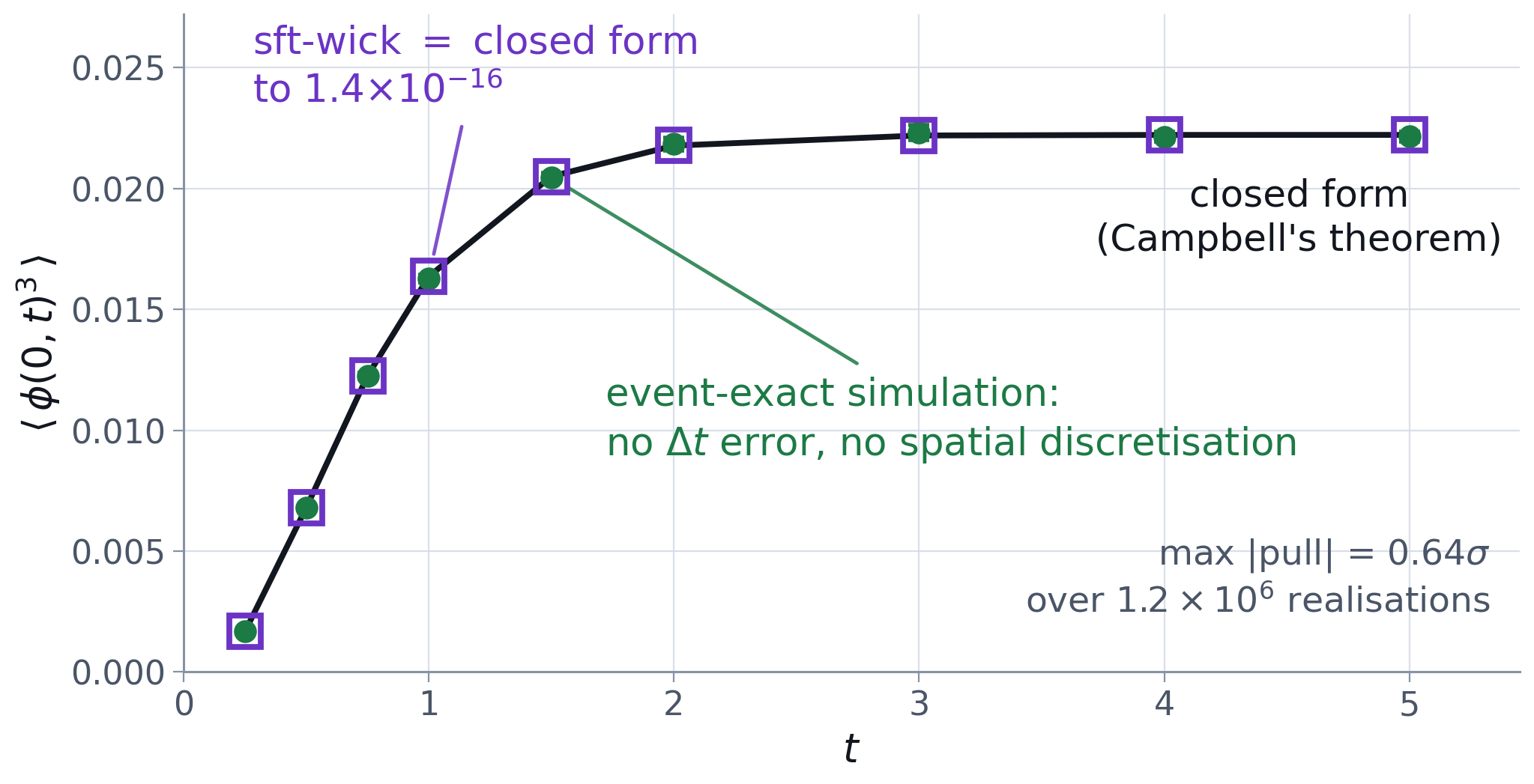
Where truth is known, we hit it exactly

third moment against time: closed form, sft-wick and an event-exact simulation

1.4×10⁻¹⁶

sft-wick vs closed form
machine precision

0.64σ

vs an event-exact simulation
no time-step error, no grid

switch off the dynamical coupling: the series terminates, the m-point function is one diagram · 1.2×10⁶ realisations

Part 2 · Non-Gaussian demo · the knob

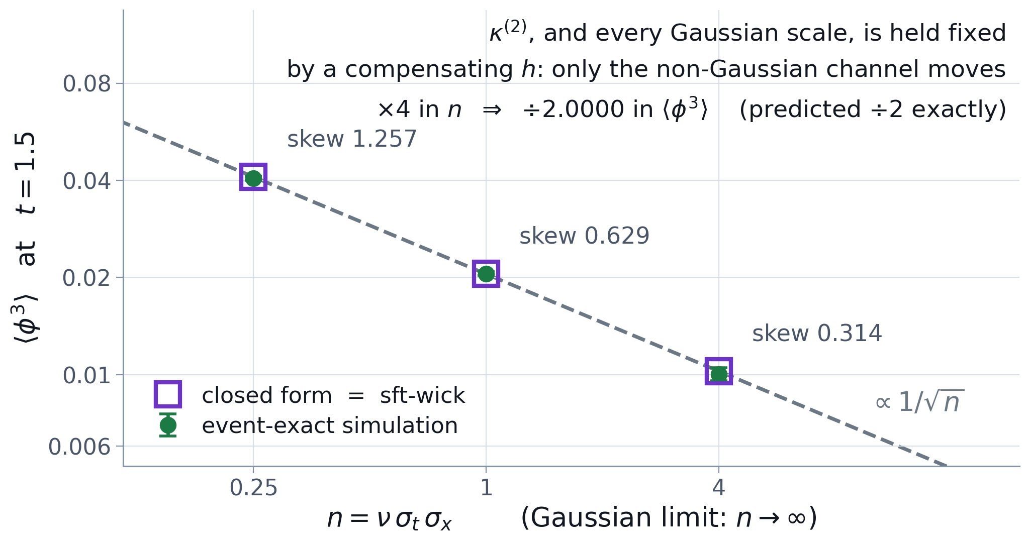
One dial moves the non-Gaussianity and nothing else

\(n \equiv \nu\,\sigma_t\,\sigma_x\) events per correlation volume · large \(n\) is the Gaussian limit: many small kicks instead of few large ones

Turning \(n\) at fixed \(\kappa^{(2)}\): the width never moves, only the shape.

third moment scaling as one over root n while the variance is held fixed

And the law it follows: \(\langle\phi^3\rangle \propto 1/\sqrt{n}\), closed form and simulation.

closed form, sft-wick and the event-exact simulation, at n = 0.25, 1, 4 · residuals within 0.8σ

Part 2 · Non-Gaussian demo · the leak

A two-point function that is pure non-Gaussianity

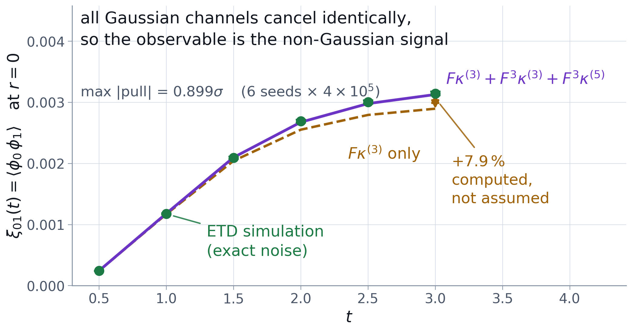
the cross-correlation xi01 against time: leading channel, full sum, and simulation

Turn the coupling back on and pick \(\xi_{01}=\langle\phi_0\phi_1\rangle\).

The drift is symmetric under \(\phi_1\to-\phi_1\). If the noise were too, \(\xi_{01}\) would vanish.

Every Gaussian channel cancels identically.

0.9σ

theory vs simulation, all six times

\(\xi_{01}=F\kappa^{(3)} + F^3\kappa^{(3)} + F^3\kappa^{(5)} + \mathcal O(F^5)\) · order 0, FF, FFFF and the whole \(\kappa^{(4)}\) channel cancel identically

[The payoff of the whole middle section.] Now turn the coupling back on, and choose the observable carefully. The drift has a symmetry: it is invariant under flipping the sign of the second component. If the noise were symmetric too, this cross-correlation would be exactly zero. It is not zero, because shot noise is skewed. So this two-point function is driven by the odd cumulants alone. Order zero cancels. The Gaussian order-two channel cancels. The entire four-cumulant channel cancels. Identically — not numerically small, algebraically zero. There is no Gaussian background here to subtract off: the observable is the non-Gaussian signal. And the prediction sits on the simulation to within one standard error at every time. That is the effect from slide four, isolated, and confirmed against a direct simulation of the same equation.

Part 3 · Insight A

The textbook kernel is the leading diagram

\[ \mathcal K(\lambda,\lambda_s)=\bar D^2\!\!\int_\lambda^{\lambda_s}\!\frac{d\lambda_1}{\bar D^2} = a^2\frac{\chi(\chi_s-\chi)}{\chi_s} \]

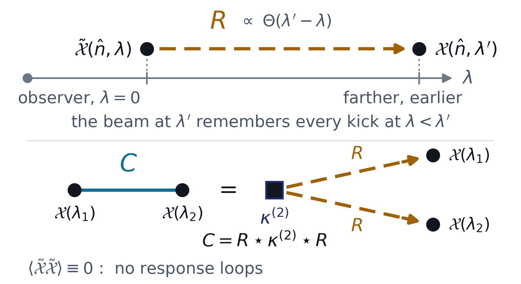
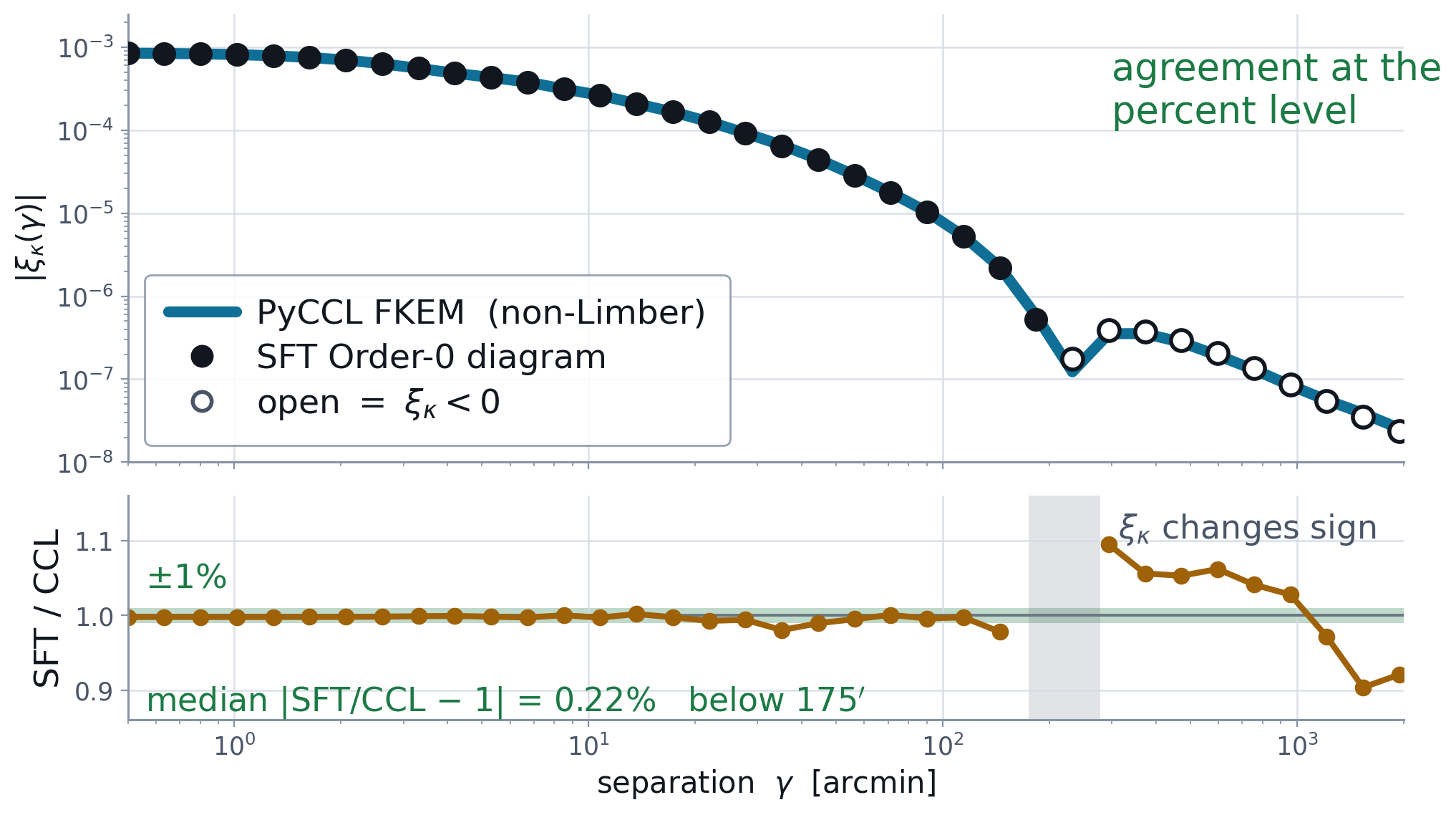
Falls out of Order-0 with no Limber, no equal-shell collapse, no flat-sky step.

The workhorse of every Stage-IV forecast is one connected diagram of this expansion, and an expansion has a next term.

Order-0 against an independent non-Limber calculation

Against PyCCL's independent non-Limber FKEM integrator, \(\gamma\in[0.5',2000']\).

percent-level agreement across four 2PCFs; largest residuals at the sign-flip zero crossings

[Deliver this flatly; the flatness is the point.] Compute the leading term. Fold the correlation propagator through the line-of-sight integrals that define the convergence, swap the order of integration, and what comes out is this — the lensing efficiency kernel. a-squared times chi times chi-s minus chi over chi-s. The textbook expression. And it comes out with no Limber approximation, no equal-shell collapse, no flat-sky step; those are extra approximations you can choose to make afterwards. So the workhorse behind every Stage-IV forecast is not a separate model — it is the leading connected diagram of one systematic expansion. On the right it is checked against PyCCL's independent non-Limber integrator: percent level over three and a half decades in angle, with the worst residuals sitting where the amplitude crosses zero, as you would expect. The reason to care is what comes next: an expansion has a second term.

Part 3 · Insight B

Which statistic can reach which observable, and at what cost

driving-field cumulants on the left, observables on the right, each route labelled with its order and vertex string

\[ \textstyle\sum_n n\,k_n \le p + k_F, \quad p + k_F + \sum_n n\,k_n \in 2\mathbb{Z} \]

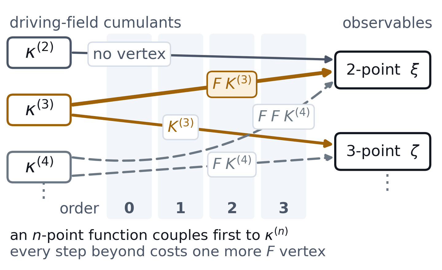
The hierarchy. A driving-field \(n\)-cumulant can feed observables of different order. Every step its index runs ahead of the observable’s costs one more \(F\) vertex, so one higher order.

The rule. At fixed order an \(n\)-point observable couples to exactly one cumulant: \(\kappa^{(n)}\) leading, \(\kappa^{(n+1)}\) through one \(F\). Higher ones have no diagram at all until higher order.

For \(\xi\) this singles out \(\kappa^{(3)}\), the bispectrum, as the one leading non-Gaussian contributor.

the exclusion is combinatorial, so it holds for any system of this shape, not just lensing

[The structural payoff. Walk the figure left to right.] This is the part that transfers, so it is the one to keep. Two halves. A mixing hierarchy: a driving-field n-cumulant can feed observables of different order, but the further its index runs ahead of the observable's, the more F vertices you need to absorb the difference, and each one costs an order. The columns are the orders, so you can count the F's. The three-cumulant reaches the three-point at order one and the two-point only at order two. The four-cumulant, dashed, is a further order back again. And the flip side, a selection rule: at fixed order an n-point observable couples to exactly one cumulant. Higher ones are not small, they are absent. There is no diagram. For the two-point function that singles out the bispectrum as the one leading non-Gaussian contributor. This is combinatorics, not a modelling choice, so it tells you which matter statistic can contaminate which lensing measurement before you compute anything.

Part 3 · The 2PCF at Order 2

At the next order, exactly two diagrams survive

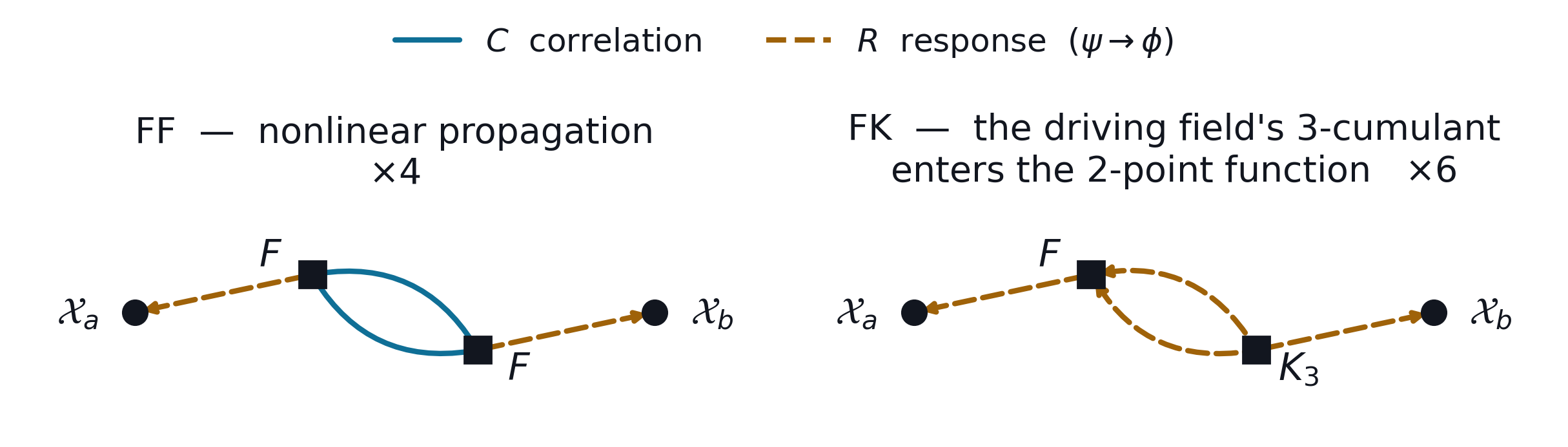
Apply that rule to the lensing 2PCF at second order.

the two surviving order-2 topologies for the lensing 2PCF

FF
there even in a Gaussian universe

FK
the matter 3-point function inside the 2-point signal

the rule kills KK and every \(K_{n\ge4}\), so these are all the Order-2 diagrams there are | generally: an \(n\)-point observable’s leading contamination is the \((n{+}1)\)-point cumulant through one \(F\) vertex

Part 3 · The number

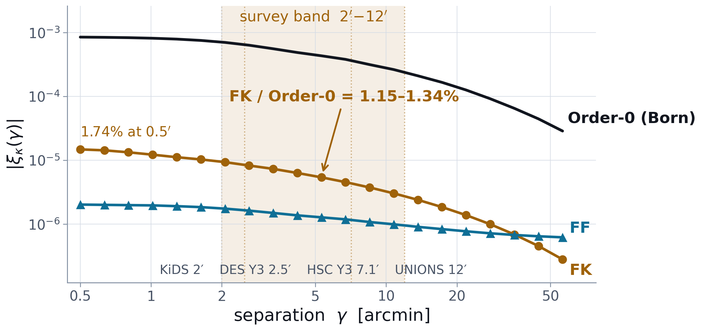
It lands inside the survey band

Order-0, FF and FK against angular separation with the survey band shaded

1.15–1.34%

FK / Order-0 across the band
KiDS 2′ · DES Y3 2.5′ · HSC 7.1′ · UNIONS 12′

Sampled in its collapsed configuration, so small-scale modes feed every separation.

\(z_s{=}5\), tree-level bispectrum, \(\ell_{\max}{=}15360\), vertex rebuilt at \(n_\phi{=}512\) with the pair-phase fix (2026-09-06; leg-symmetry 864/864 pass). Quoted for \(\gamma\lesssim1^\circ\).

Part 3 · How solid, and how to find it

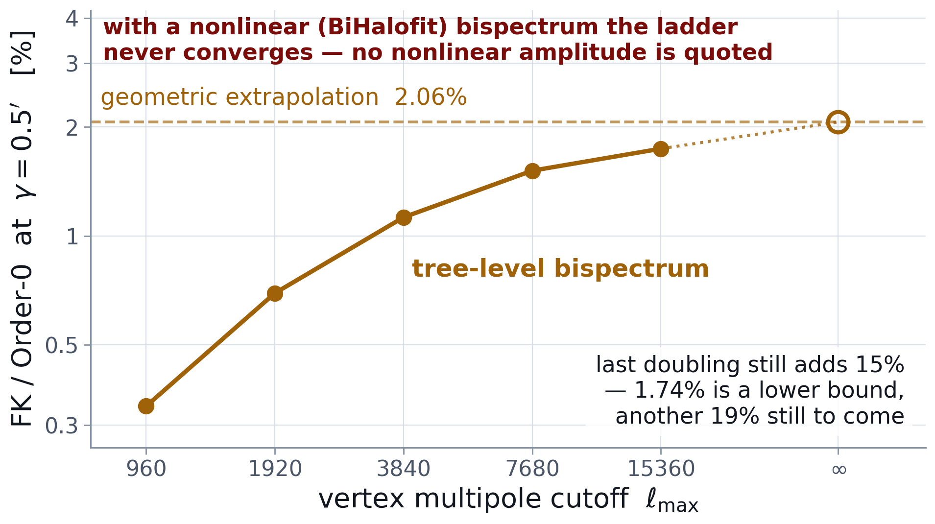
Still climbing, and it has a signature

FK amplitude against multipole cutoff, still rising

A coincident-point moment is UV-sensitive by construction. The quoted amplitude is a floor.

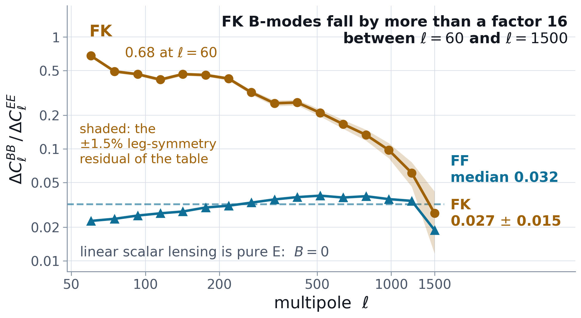
FK B-mode to E-mode ratio against multipole

Linear scalar lensing is pure E, so any B at this level is Order-2. FK’s falls steeply with \(\ell\) and crosses FF near \(\ell\sim1100\); the shaded band is the vertex table’s own residual.

\(\Delta C_\ell^{EB}=0\) exactly, by parity | FK/O0 at 0.5′ also grows monotonically with source redshift, 1.06% at \(z_s{=}1\) to 1.76% at \(z_s{=}5\)

[Two panels, thirty seconds each.] Left: honesty. A collapsed configuration is a coincident-point moment, so it is ultraviolet-sensitive by construction. That is physics, not bookkeeping. The amplitude is still climbing: the last doubling adds fifteen per cent and an extrapolation says another nineteen, so treat the number as a floor with a known direction of travel. With a nonlinear bispectrum it does not converge at all, which is why I quote no nonlinear amplitude. Right: how you would find it. Linear scalar lensing is pure E-mode, a theorem, so any B-mode at this level is second order and both second-order terms make some. FK starts near two thirds of E at ell of sixty and falls steeply, crossing FF around ell of eleven hundred, where FF sits flat at three per cent. The shape is the signature, not the amplitude. [The shaded band is the vertex table's own leg-symmetry residual propagated through. It is invisible at low ell and swallows the last two points, so do not quote the high-ell value as a number. The parity null is a different kind of statement and carries no band: the EB cross-spectrum is identically zero, by parity, not numerically.] It also grows with source redshift, which gives you a second handle. [If time is short, cut the redshift sentence.]

Take-aways

Three things to remember

Nonlinear dynamics plus a non-Gaussian drive let an \((n{+}1)\)-point statistic reach an \(n\)-point observable. The MSR diagrammatics counts it, and sft-wick does the counting for you.
Where the truth is known, the machine hits it to machine precision, including a two-point function that is pure non-Gaussianity, with every Gaussian channel cancelling identically.
In weak lensing the textbook projection is Order-0. The next term puts the matter bispectrum into the two-point signal at the per-cent level inside the survey band, with a B-mode signature.

Supported by ERC

sft-wick: pip install sft-wick · docs sft-wick.readthedocs.io · arXiv:2606.19480 | lensing: arXiv:2606.19472

[Land it and stop. Do not add a fourth point.] Three things. One: when a nonlinear system is driven by a non-Gaussian field, the higher statistics do not stay put — they reach down into the lower ones, and the MSR diagrammatics is the bookkeeping that tells you exactly how much. sft-wick does that bookkeeping automatically, and it is on PyPI. Two: where I can construct a case with a known exact answer, the machine hits it to machine precision — including a two-point function whose entire content is non-Gaussian, because every Gaussian channel cancels algebraically. Three: applied to weak lensing, the textbook projection turns out to be the leading diagram, and the next term carries the matter bispectrum into the two-point signal at the per-cent level right in the band the surveys use — with a B-mode signature that distinguishes it. Thank you.

Backup

Backup slides

Press ↓ to page through, → to skip out.

Monte-Carlo validation of the FK diagram
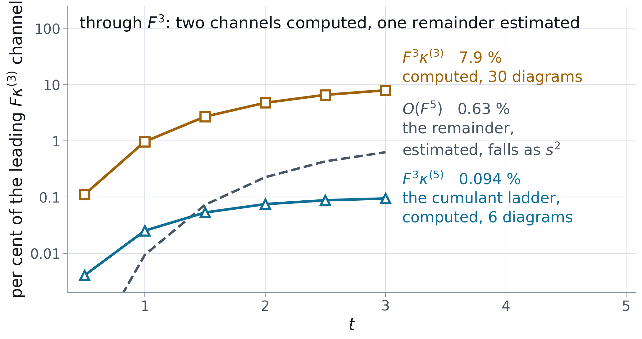
The non-Gaussian error budget: what is computed, what is left
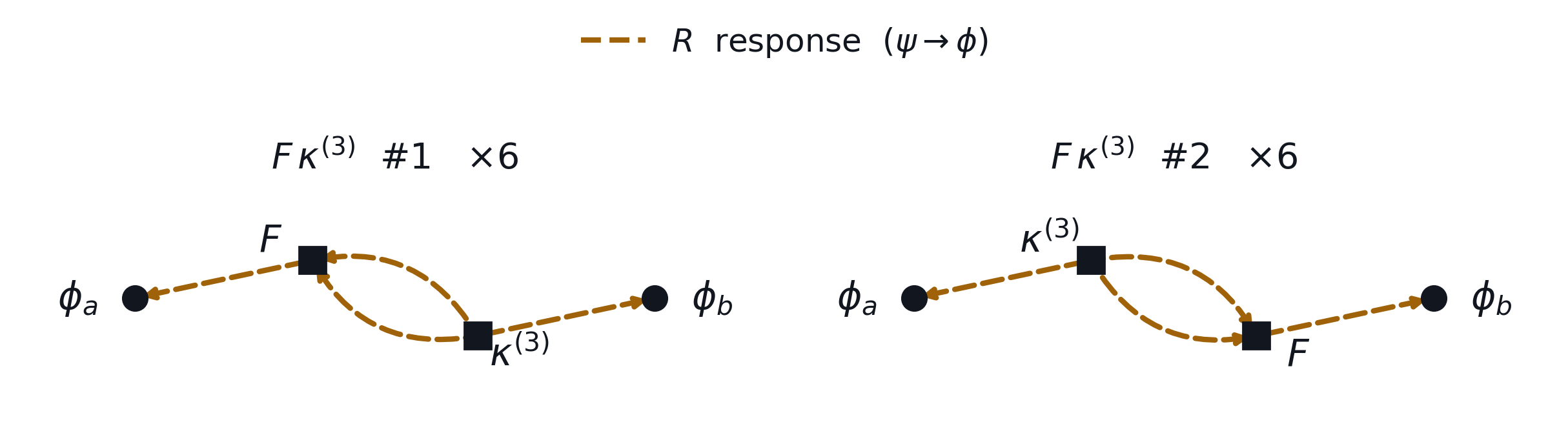
The two \(F\kappa^{(3)}\) diagrams of the toy model
Where the FK number is still moving
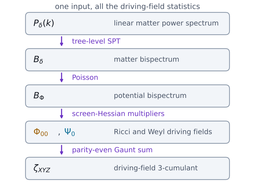
Driving-field statistics from one input \(P_\delta(k)\)

Backup · validation

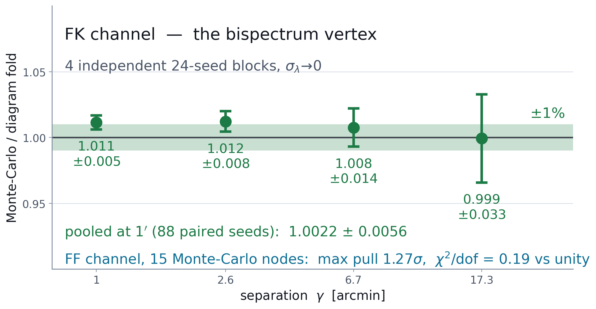
FK against direct simulation

Monte-Carlo over analytic ratio against separation

Monte-Carlo integration of the stochastic Sachs equation, independent of the diagrammatic expansion. Ratio to the analytic fold: 1.011 ± 0.005 at 1′, consistent with unity out to 17′.

corrected estimator (2026-08-28); the earlier variance-reduced estimator was withdrawn

Backup · the toy model

What is computed, and what is left

error budget: computed channels and the estimated remainder

The \(\kappa^{(5)}\) ladder is computed at 0.09% of the leading channel. One named remainder is left, \(\mathcal O(F^5)\), estimated geometrically at 0.63%.

Backup · the toy model

The two diagrams behind the leak

No correlation propagator appears at all: the signal is response legs running into a cumulant vertex.

Backup · caveats

Where the FK number is still moving

UV convergence.
Still rising with \(\ell_{\max}\); geometric extrapolation adds ~19%. No nonlinear-bispectrum amplitude is quoted, because that sum does not converge.

Vertex table.
Two defects found and fixed (2026-09-06): a dropped pair phase, and \(n_\phi\) under-integration. Rebuilt; the leg-symmetry test went 864/864 fail to 864/864 pass.

Angular range.
Quoted only for \(\gamma\lesssim1^\circ\): beyond that the multipole sum oscillates and does not converge.

Approximations in the run.
Scalar-only, \(\Phi=\Psi\), Born path, single source plane, tree-level SPT bispectrum.

If someone pushes on the number, this is the slide. Four things. The multipole sum is still climbing, and a geometric extrapolation adds about nineteen per cent — so the quoted value is a floor. The vertex table behind it had two defects; both are now fixed and the table rebuilt, which is where these numbers come from. The net was a downward shift of about a quarter: one point seven four per cent at half an arcminute where the old table said two point three one. The acceptance test is a symmetry the vertex must satisfy exactly, and it went from failing every cell to passing every cell. The angular range is restricted to about a degree for a convergence reason, not a physics one. And the numerical run is scalar-only on a Born path with a tree-level bispectrum. The structure — the selection rule, Order-0 being the textbook kernel, FK existing at all — none of that depends on any of these.

Backup · inputs

Driving-field statistics from one input

from the matter power spectrum to the driving-field cumulants

\(P_\delta \rightarrow B_\delta\) (tree-level SPT) \(\rightarrow B_\Phi\) (Poisson) \(\rightarrow (\Phi_{00},\Psi_0)\) via screen-Hessian multipliers \(\rightarrow \zeta_{XYZ}\) by a parity-even Gaunt sum.

exact Wigner-3j below \(\ell=60\), Limber above; FFTlog double-Bessel radial integrals