sft-wick

Stochastic fields · Feynman diagrams · Python

sft-wick

Feynman-diagram expansion and evaluation in stochastic field theories

Computer Physics Communications Seminar Series6 November 2026

Zheng Zhang

Jodrell Bank Centre for Astrophysics, University of Manchester

pip install sft-wickgithub.com/StatFieldTheory/sft-wick

A system of stochastic differential equations

$$\begin{aligned}\partial_t\varphi_1 &= \hl{b}{-\varphi_1} + \hl{c}{\varphi_2^2} + \hl{d}{\eta_1}\\[6pt] \partial_t\varphi_2 &= \hl{b}{-\varphi_2} + \hl{c}{\varphi_1\varphi_2} + \hl{d}{\eta_2}\end{aligned}$$

$$\vev{\hl{d}{\eta_a(x,t)}\,\hl{d}{\eta_b(x',t')}} = \delta_{ab}\,\lambda\,e^{-|t-t'|/\sigma_t}\,e^{-|x-x'|/\sigma_x}$$

linear decayquadratic couplingrandom driving field

sft-wick computes, order by order

$$\vev{\varphi_a(x,t)\,\varphi_b(y,t)} = \xi^{(0)}_{ab} + \xi^{(2)}_{ab} + \xi^{(4)}_{ab} + \cdots$$

Fields \(\varphi_{1,2}(x,t)\) on a line: worked example I of the paper

With support from

ERC grant agreement No. 948764  ·  RadioForegroundsPlus GA 101135036

This talk is about sft-wick, a Python package for stochastic field equations such as the pair on the right: two fields on a line, each decaying, coupled quadratically and driven by random noise. It builds the Feynman-diagram expansion of such a system and evaluates the diagrams numerically, order by order. I will derive the expansion, run a calculation from a YAML file, and show two applications: non-Gaussian noise and weak lensing.

We want the statistics of a noise-driven field

sft-wick

1. 01 Formalism
2. 02 Hands-on
3. 03 Non-Gaussian
4. 04 Lensing

We want the statistics of a noise-driven field

Driveone realisation of \(\eta_1, \eta_2\) at a point

Fieldthe equations on the cover, integrated in time

Ensemble80 of 5 000 realisations; mean, \(\pm1\sigma\), and the distribution for \(t \ge 5\)

The target

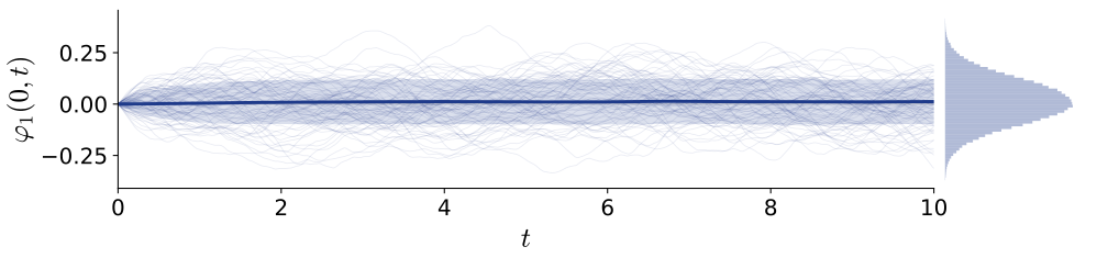
Averages over realisations: \(\vev{\varphi_a}\), \(\vev{\varphi_a\varphi_b}\), \(\vev{\varphi_a\varphi_b\varphi_c}\), …

Averages do not close

$$\partial_t\vev{\varphi_1} = -\vev{\varphi_1} + \vev{\varphi_2^2}$$

Each \(n\)-point function needs the \((n{+}1)\)-point function: the closure problem from turbulence that the MSR formalism organises.

The same structure appears in

turbulencestochastic inflationstructure formationcritical dynamicsneural networksweak lensing

Worked example I at one point: exact AR(1) drive, Heun steps, as in examples/demo1 · applications: paper, Sec. 1

Here is what the equations on the cover do. Take one point in space. The top panel is one realisation of the two driving fields there. Integrating the equations in time turns it into one history of the two fields: smoother, because the field remembers earlier kicks, and coupled through the quadratic terms.

A new realisation of the noise gives a new history. What we want is not one history but averages over many: the mean, the two-point function, and so on. The bottom panel shows eighty of five thousand simulated histories.

Why not average the equation directly? It does not close. The mean of phi-one depends on the average of phi-two squared, a two-point function, which in turn depends on a three-point function. This is the closure problem of turbulence, where the response-field formalism began. The same structure appears in cosmology, critical dynamics and neural networks.

Two random drives with the same covariance

sft-wick

1. 01 Formalism
2. 02 Hands-on
3. 03 Non-Gaussian
4. 04 Lensing

Two random drives with the same covariance

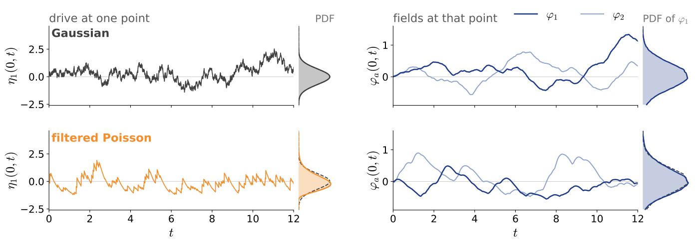
Drives: same mean and \(\cumulant^{(2)}\). Only the lower one has \(\cumulant^{(3)}, \cumulant^{(4)}, \dots\)
Fields: same variance. Skewness 0.00 and 0.34 (4 000 runs).
Worked example II: the cover's equations, coupling \(\times\,0.2\).

Through the nonlinear dynamics, does the difference reach a two-point function \(\vev{\varphi\varphi}\)? By how much, and through which terms?

Now the question for this talk. Here are two drives at one point, with the same mean and the same two-point cumulant. The upper one is Gaussian. The lower one is shot noise: random events, each followed by a decaying pulse. It is skewed, and its higher cumulants are nonzero. Both drive the same nonlinear system. The last column is the distribution of phi-one over four thousand runs. The variances agree, and the shot-noise field is skewed. A linear system would pass the skewness on too, and would give both fields the same covariance.

So the question is the two-point function. With the nonlinearity, do the higher cumulants reach it, by how much, and through which terms? Four thousand runs measure phi-one phi-two only to plus or minus three times ten to the minus three, which does not settle it. The diagram expansion answers term by term, in part three.

Plan

sft-wick

1. 01 Formalism
2. 02 Hands-on
3. 03 Non-Gaussian
4. 04 Lensing

Plan

01

From noise to diagrams

Path integral, two propagators, Wick's theorem and Feynman rules.

11 MIN

02

A first calculation

Write the model in YAML, run it, read the output, change a parameter.

7 MIN

03

Non-Gaussian driving

Higher cumulants as vertices, and the answer to the opening question.

4 MIN

04

Weak lensing

A light bundle in a random universe, treated as a stochastic field.

5 MIN

The YAML files, commands and outputs of part 2 are in the tutorial/ folder that accompanies this recording.

Four parts. First, the formalism: path integral, propagators, Wick’s theorem and Feynman rules. Second, a first calculation from one YAML file. Third, non-Gaussian driving, which answers the opening question. Fourth, weak lensing, the motivating application.

From noise to diagrams

01

From noise to diagrams

A stochastic field equation becomes a field theory with two propagators and a set of vertices.

01 · Formalism

02 · Hands-on

03 · Non-Gaussian

04 · Lensing

Part one: from noise to diagrams.

A field driven by random noise

sft-wick

1. 01 Formalism
2. 02 Hands-on
3. 03 Non-Gaussian
4. 04 Lensing

A field driven by random noise

$$\partial_t \varphi_a(\bm{x}, t) = \underbrace{A_{ab}\,\varphi_b}_{\text{linear}} + \underbrace{\mathcal{F}_a[\varphi]}_{\text{nonlinear}} + \underbrace{\eta_a(\bm{x}, t)}_{\text{driving field}}$$

$$\mathcal{F}_a[\varphi] = F^{(3)}_{abc}\,\varphi_b\varphi_c + F^{(4)}_{abcd}\,\varphi_b\varphi_c\varphi_d + \cdots$$

The driving field is set by its cumulant generating functional:

$$\begin{aligned}W[\ii J] &= \ln\vev{e^{\ii\int J_a\eta_a\,\dd\bm{x}\,\dd t}}_{\eta}\\ &= \sum_{n\ge1}\frac{\ii^n}{n!}\int\!\cumulant^{(n)}_{a_1\cdots a_n}\,J_{a_1}\cdots J_{a_n}\end{aligned}$$

Gaussian if \(\cumulant^{(n)} = 0\) for all \(n > 2\). Zero mean is assumed.

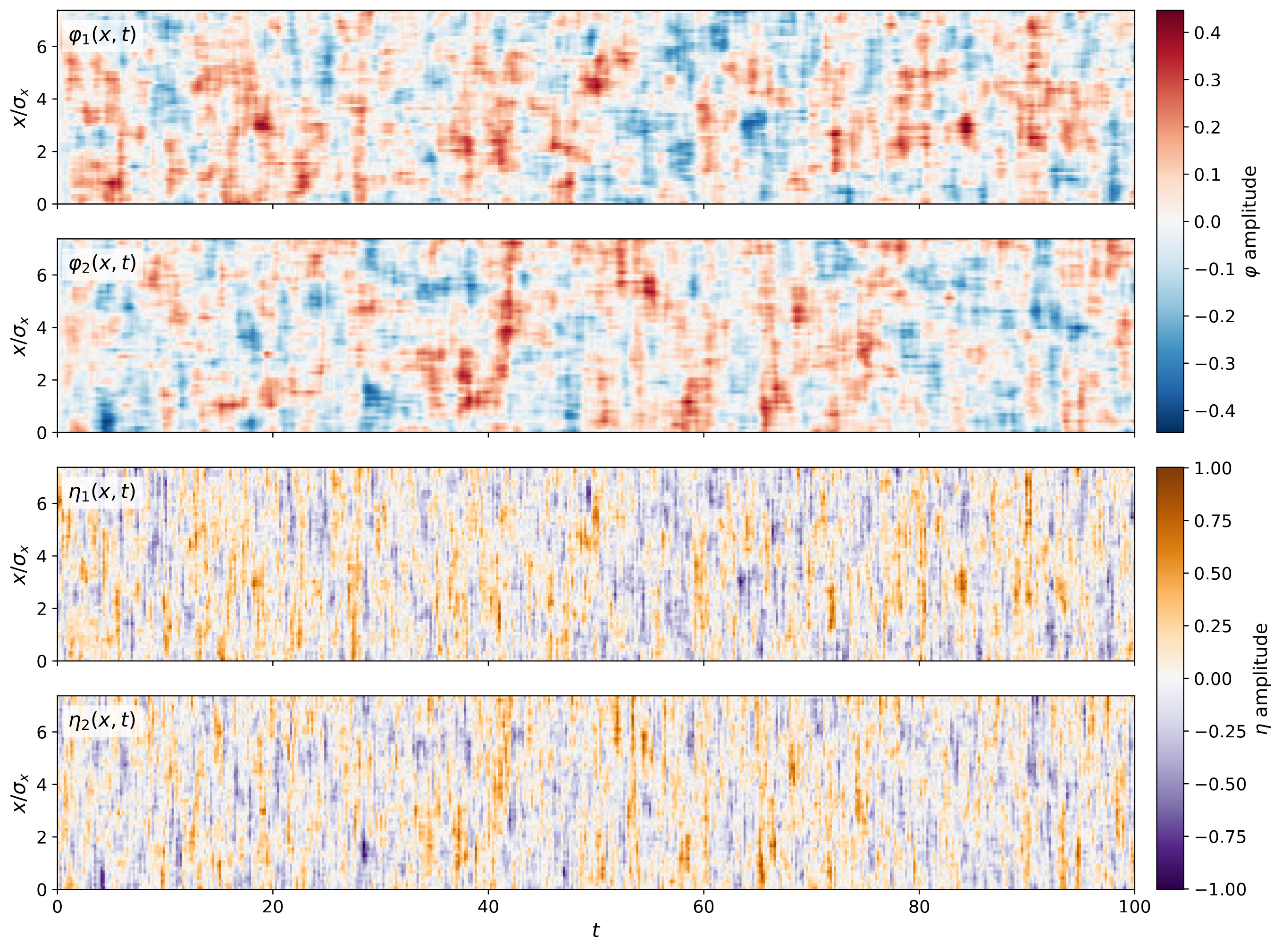
Goal: ensemble averages, such as \(\xi_{ab} = \vev{\varphi_a(\bm{x},t)\,\varphi_b(\bm{y},t)}\)

One realisation of worked example I (paper, Fig. 1): fields \(\varphi_{1,2}\), driving fields \(\eta_{1,2}\)

Now the general form. The field phi has several components, labelled a. The equation has three terms: a linear term with a matrix A; a nonlinear term F, a polynomial in the field, starting with the quadratic coupling tensor F-three; and the driving field eta.

The driving field is described by its cumulant generating functional W: the logarithm of the average of an exponential of the noise against an auxiliary current J. Expanding W in powers of J gives the cumulants. The second cumulant is the covariance; if all higher ones vanish, the drive is Gaussian. We take the mean to be zero.

On the right is the first worked example over space and time: the fields and their drives.

A response field turns the equation into a path integral

sft-wick

1. 01 Formalism
2. 02 Hands-on
3. 03 Non-Gaussian
4. 04 Lensing

A response field turns the equation into a path integral

1

$$P[\varphi] = \int\!\mathcal{D}\eta\;P[\eta]\;\delta^N\!\big[f[\varphi] - \eta\big],\qquad f[\varphi] = \partial_t\varphi - A\varphi - \mathcal{F}[\varphi]$$

Each realisation of \(\eta\) fixes one history \(\varphi\). With Itô time slicing the Jacobian is a constant.

2

$$\delta^N\!\big[f - \eta\big] = \int\!\mathcal{D}\psi\;e^{-\ii\int\psi_a\,(f_a - \eta_a)\,\dd\bm{x}\,\dd t}$$

Fourier representation: one response field \(\psi_a\) per component (Martin, Siggia, Rose).

3

$$\int\!\mathcal{D}\eta\;P[\eta]\;e^{\ii\int\psi_a\eta_a\,\dd\bm{x}\,\dd t} = e^{W[\ii\psi]}$$

The noise average is its cumulant generating functional at \(J = \psi\).

⇓

$$P[\varphi] = \int\!\mathcal{D}\psi\;e^{-S[\varphi,\psi]},\qquad S[\varphi,\psi] = \hl{a}{\ii\!\int\!\psi_a\big(\partial_t\varphi_a - A_{ab}\varphi_b - \mathcal{F}_a[\varphi]\big)\,\dd\bm{x}\,\dd t}\;-\;\hl{b}{W[\ii\psi]}$$

equation of motion, steps 1 and 2noise statistics, step 3

Paper, Sec. 2.1 · Jacobian: App. D

Three steps turn this equation into a field theory.

First: each realisation of the noise fixes one history of the field. So the probability of a field history is the average, over the noise, of a delta functional that enforces the equation of motion. In the Itô discretisation the Jacobian of this change of variables is a constant, so we can drop it.

Second: write the delta functional as a Fourier integral. This introduces a new field psi, one for each component, conjugate to the equation of motion. It is the response field of Martin, Siggia and Rose.

Third: the noise now appears only in the exponential of i psi times eta. Its average is, by definition, the cumulant generating functional W, evaluated at J equal to psi.

The result is a path integral over psi, with an action S. The first term, in blue, comes from the equation of motion. The second, in amber, carries all the statistics of the noise.

Split the action and expand in the interaction

sft-wick

1. 01 Formalism
2. 02 Hands-on
3. 03 Non-Gaussian
4. 04 Lensing

Split the action and expand in the interaction

$$\vev{O[\varphi]}_S = \frac{1}{Z_S}\int\!\mathcal{D}\varphi\,\mathcal{D}\psi\;O[\varphi]\,e^{-S[\varphi,\psi]},\qquad S = S_0 + \Sint,\qquad Z_S = 1$$

Free part \(S_0\): Gaussian

$$S_0 = \ii\!\int\!\psi_a\big(\partial_t\varphi_a - A_{ab}\varphi_b\big)\,\dd\bm{x}\,\dd t \;-\; W_{\mathrm{G}}[\ii\psi]$$

Linear dynamics and the second cumulant \(\cumulant^{(2)}\). Quadratic in \(\varphi\) and \(\psi\).

Interaction \(\Sint\): vertices

$$\Sint = -\ii\!\int\!\psi_a\,\mathcal{F}_a[\varphi]\,\dd\bm{x}\,\dd t \;-\; W_{\mathrm{NG}}[\ii\psi]$$

• \(-\ii\,F^{(3)}_{abc}\,\psi_a\varphi_b\varphi_c\): one point, one \(\psi\) and two \(\varphi\)
• \(\tfrac{\ii}{3!}\,\cumulant^{(3)}_{abc}\,\psi_a\psi_b\psi_c,\ \dots\): legs at distinct points (part 3)

$$\vev{O}_S = \sum_{n=0}^{N}\frac{(-1)^n}{n!}\,\vevfree{O\,\Sint^n}$$

Order \(n\) is the number of vertices. Every term is a moment of the Gaussian theory \(S_0\).

Paper, Sec. 2.2 · \(Z_S = 1\): App. D

The average of an observable O is a path integral with the weight e to the minus S. The normalisation Z-S is exactly one for any nonlinearity under the Itô prescription, so there are no vacuum diagrams to subtract.

The integral cannot be done exactly, so we split the action in two. The free part S-zero contains the linear dynamics and the Gaussian part of the noise, the second cumulant. It is quadratic in phi and psi. The interaction part contains everything else. The nonlinearity gives a local vertex: one psi and two phi fields at the same point, with coupling F. The cumulants of order three and higher give vertices made of psi fields only, at different points. We come back to those in part three.

Expanding the exponential of the interaction gives the series at the bottom. The order n is the number of vertices, and every term is a moment of the Gaussian theory.

The Gaussian part is fixed by two propagators

sft-wick

1. 01 Formalism
2. 02 Hands-on
3. 03 Non-Gaussian
4. 04 Lensing

The Gaussian part is fixed by two propagators

\(S_0\) as a quadratic form

$$S_0 = \frac12\begin{pmatrix}\varphi^T & \psi^T\end{pmatrix}\begin{pmatrix}0 & \ii\DeterOp^T\\[3pt] \ii\DeterOp & \cumulant\end{pmatrix}\begin{pmatrix}\varphi\\[3pt] \psi\end{pmatrix}$$

$$\DeterOp_{ab}(\bm{x}',t';\bm{x},t) = \delta(\bm{x}'-\bm{x})\,\delta(t'-t)\,\big[\delta_{ab}\partial_t - A_{ab}\big]$$

→

Its inverse

$$G_0 = \begin{pmatrix}\hl{C}{\CorrOp} & \hl{R}{-\ii\RespOp}\\[3pt] \hl{R}{-\ii\RespOp^T} & \hl{z}{0}\end{pmatrix}$$

$$\RespOp = \DeterOp^{-1},\qquad \CorrOp = \RespOp\,\cumulant\,\RespOp^T$$

Correlation

$$\vevfree{\varphi_a(\bm{x})\,\varphi_b(\bm{y})} = \CorrOp_{ab}(\bm{x};\bm{y})$$

Solid line, no direction.

Response

$$\vevfree{\varphi_a(\bm{x})\,\psi_b(\bm{y})} = -\ii\,\RespOp_{ab}(\bm{x};\bm{y})$$

Dashed line, arrow from \(\psi\) to \(\varphi\).

No \(\psi\psi\) line

0

$$\vevfree{\psi_a(\bm{x})\,\psi_b(\bm{y})} = 0$$

Every \(\psi\) must pair with a \(\varphi\).

Paper, Sec. 2.3 · \(\bm{x}, \bm{y}\): space-time points · same structure as the classical limit of the Schwinger–Keldysh formalism, with \(G^{qq} = 0\)

The free action is quadratic, so the free theory is a Gaussian integral, fixed by its two-point functions. Write S-zero as a quadratic form in the pair phi and psi. The matrix has zero in the phi-phi block, the linear operator D in the off-diagonal blocks, and the noise covariance K in the psi-psi block. D is the time derivative minus A.

Inverting this matrix gives the propagators. The response propagator R is the inverse of D, the Green’s function of the linear dynamics. The correlation propagator C is R K R-transpose: the noise covariance, carried by the linear dynamics to both points.

Below are the three two-point functions, drawn as in the package and the paper. Phi-phi is C, a solid blue line. Phi-psi is minus i R, a red dashed line with an arrow from psi to phi. And psi-psi vanishes. There is no such line, so every psi must pair with a phi.

Both propagators follow from the linear dynamics

sft-wick

1. 01 Formalism
2. 02 Hands-on
3. 03 Non-Gaussian
4. 04 Lensing

Both propagators follow from the linear dynamics

Response \(\RespOp = \DeterOp^{-1}\)

$$\RespOp_{ab}(\bm{x},t;\bm{x}',t') = \delta(\bm{x}-\bm{x}')\,\Theta(t-t')\,\Big\{\mathcal{T}\!\exp\!\int_{t'}^{t}\!\mathbf{A}(\bm{x},\tau)\,\dd\tau\Big\}_{ab}$$

• Retarded: zero for \(t \le t'\), with the Itô value \(\Theta(0) = 0\).
• Local in \(\bm{x}\): each \(\RespOp\) line removes one spatial integral.

Worked example I, \(A_{ab} = -\delta_{ab}\)

$$\RespOp_{ab}(x,t;x',t') = \delta(x-x')\,\Theta(t-t')\,e^{-(t-t')}\,\delta_{ab}$$

Correlation \(\CorrOp = \RespOp\,\cumulant\,\RespOp^T\)

$$\CorrOp_{ab}(\bm{z}_1;\bm{z}_2) = \int\!\dd\bm{z}'\,\dd\bm{z}''\;\RespOp_{ad}(\bm{z}_1;\bm{z}')\,\cumulant_{dc}(\bm{z}';\bm{z}'')\,\RespOp_{bc}(\bm{z}_2;\bm{z}'')$$

• Symmetric: \(\CorrOp_{ab}(\bm{z};\bm{z}') = \CorrOp_{ba}(\bm{z}';\bm{z})\), with \(\bm{z} = (\bm{x}, t)\).
• The noise covariance, carried to both points by the linear dynamics.

Worked example I: closed form, built in

$$\begin{aligned}\CorrOp_{ab}(x,t;x',t') ={}& e^{-|x-x'|/\sigma_x}\,\delta_{ab}\\ &\times\int_{0}^{t}\!\dd\tau\!\int_{0}^{t'}\!\dd\tau'\;\lambda\,e^{-|\tau-\tau'|/\sigma_t}\,e^{-(t-\tau)}\,e^{-(t'-\tau')}\end{aligned}$$

Paper, Sec. 2.4 · worked example I: Sec. 3

Explicitly, R is a delta function in space, a step function in time, and the time-ordered exponential of A. It is retarded: the field does not respond to noise from the future, and with the Itô convention it also vanishes at equal times. It is local in space, so each R line in a diagram removes one spatial integral.

C is two responses joined by the noise covariance, and it is symmetric under exchange of its two points.

In the worked example A is minus the identity. Then R is a decaying exponential, and C is a double time integral of the noise kernel. That integral has a closed form in elementary functions, which the package has built in. We use it in part two.

Wick’s theorem: each pairing is a product of propagators

sft-wick

1. 01 Formalism
2. 02 Hands-on
3. 03 Non-Gaussian
4. 04 Lensing

Wick's theorem: each pairing is a product of propagators

$$\vev{X_1X_2\cdots X_{2n}} = \sum_{p\,\in\,P^2_n}\;\prod_{\{i,j\}\in p}\vev{X_iX_j}$$

Gaussian fields: sum over the \((2n-1)!!\) ways to split \(2n\) fields into pairs.

Order 2 of \(\vev{\varphi_a(\bm{x})\,\varphi_b(\bm{y})}\): two cubic vertices at \(\bm{z}_0\) and \(\bm{z}_1\)

$$\vevfree{\varphi_a(\bm{x})\,\varphi_b(\bm{y})\,\Sint^2} = (-\ii)^2\!\int\!\dd\bm{z}_0\,\dd\bm{z}_1\,F^{(3)}_{cde}F^{(3)}_{fgh}\,\vevfree{\hl{b}{\varphi_a(\bm{x})}\,\hl{e}{\varphi_b(\bm{y})}\;\hl{b}{\psi_c(\bm{z}_0)}\,\hl{c}{\varphi_d(\bm{z}_0)}\,\hl{d}{\varphi_e(\bm{z}_0)}\;\hl{e}{\psi_f(\bm{z}_1)}\,\hl{c}{\varphi_g(\bm{z}_1)}\,\hl{d}{\varphi_h(\bm{z}_1)}}$$

One of the \(7!! = 105\) pairings

$$\hl{b}{\vevfree{\varphi_a(\bm{x})\,\psi_c(\bm{z}_0)}}\;\hl{e}{\vevfree{\varphi_b(\bm{y})\,\psi_f(\bm{z}_1)}}\;\hl{c}{\vevfree{\varphi_d(\bm{z}_0)\,\varphi_g(\bm{z}_1)}}\;\hl{d}{\vevfree{\varphi_e(\bm{z}_0)\,\varphi_h(\bm{z}_1)}}$$

$$= (-\ii)^2\;\RespOp_{ac}(\bm{x};\bm{z}_0)\,\RespOp_{bf}(\bm{y};\bm{z}_1)\,\CorrOp_{dg}(\bm{z}_0;\bm{z}_1)\,\CorrOp_{eh}(\bm{z}_0;\bm{z}_1)$$

The same term, drawn by sft-wick: diagram (b) of paper Fig. 2

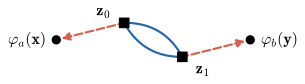
Of the 105 pairings, 30 are nonzero. They fall into 6 topologies; diagram (b) collects \(\mu = 4\) of them.

Every term of the series is a Gaussian moment, and Wick’s theorem evaluates it. The average of a product of 2n Gaussian fields is the sum, over all ways of splitting the fields into pairs, of products of two-point functions. There are 2n minus 1 double-factorial such pairings.

Take the second-order term of the two-point function. Two copies of the cubic vertex, at points z-zero and z-one, each bring one psi and two phi fields. With the two external fields that makes eight fields, and 105 pairings.

Here is one of them, colour-coded. The external phi at x pairs with the psi at z-zero, and the one at y with the psi at z-one: two response propagators. The four remaining phi fields pair across the two vertices: two correlation propagators. The product is this term. On the right is the same term as a diagram, drawn by the package.

Most of the 105 pairings vanish. The 30 that do not fall into six topologies, and this one collects four of them.

Feynman rules: one diagram, one integral

sft-wick

1. 01 Formalism
2. 02 Hands-on
3. 03 Non-Gaussian
4. 04 Lensing

Feynman rules: one diagram, one integral

Feynman rules

	\(\CorrOp(\bm{z};\bm{z}')\)
	\(-\ii\,\RespOp(\bm{z};\bm{z}')\), from \(\psi\) to \(\varphi\)
	\(-\ii\,F^{(3)}\) and \(\int\!\dd\bm{z}\) over the vertex
	external field \(\varphi_a(\bm{x})\)
order \(n\)	\(\dfrac{(-1)^n}{n!}\) and the multiplicity \(\mu\)

Odd orders vanish: \(3n+2\) fields cannot all be paired when \(n\) is odd.

Order 0 and order 2 of \(\vev{\varphi_a\varphi_b}\) (paper, Fig. 2)

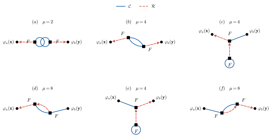
Diagram (b): \(\displaystyle\int\!\dd\bm{z}_0\,\dd\bm{z}_1\;\RespOp(\bm{x};\bm{z}_0)\,\RespOp(\bm{y};\bm{z}_1)\,\CorrOp(\bm{z}_0;\bm{z}_1)\,\CorrOp(\bm{z}_0;\bm{z}_1)\), with coefficient and coupling sum set by the rules.

Paper, Sec. 2.8 and Sec. 3.2

These are the Feynman rules. A solid line is a C propagator. A dashed line is minus i R, pointing from psi to phi. A square is a vertex, with a factor minus i F and an integral over its position and time. A circle is an external field. At order n there is an overall factor minus one to the n over n factorial, and each topology carries its multiplicity mu.

On the right are the diagrams up to second order, as in the paper. Order zero is a single C line. Odd orders vanish, because three n plus two fields cannot all be paired. Order two has six topologies. Each is one integral; diagram b is the one we built on the previous slide.

Three rules remove most Wick pairings

sft-wick

1. 01 Formalism
2. 02 Hands-on
3. 03 Non-Gaussian
4. 04 Lensing

Three rules remove most Wick pairings

Order 2 of \(\vev{\varphi_a\varphi_b}\): 105 pairings

1. No \(\psi\psi\) pairs\(\vevfree{\psi\psi} = 0\).−15
2. Itô convention\(\Theta(0) = 0\), so \(\RespOp(\bm{x},t;\bm{x}',t) = 0\): no \(\varphi\psi\) pair at one vertex.−48
3. CausalityA closed loop of \(\RespOp\) lines needs \(t_1 \ge t_2 \ge \cdots \ge t_1\).−12

30 pairings remain, in 6 topologies.

Cubic vertex, \(N = 3\) components (paper, Table 2)

\(n = 1\)\(\vev{\varphi\varphi\varphi}\)

15

6

\(n = 2\)\(\vev{\varphi\varphi}\)

105

6

\(n = 3\)\(\vev{\varphi\varphi\varphi}\)

\(1.0\times10^{4}\)

80

Wick pairings \((3n+m-1)!!\) diagrams returnedlog scale

Paper, Secs. 2.5 to 2.7 · counts applied in the order listed

Three rules remove the vanishing pairings, and each is visible in the second-order example. First, no psi-psi pairs: that removes fifteen of the 105. Second, the Itô convention. A phi and a psi at the same vertex would give R at equal times, which is zero; that removes forty-eight more. Third, causality. A closed loop of R lines would need each time to be later than the next, all the way round; that removes twelve. Thirty pairings remain.

On the right, from Table 2 of the paper, is the same reduction at higher order. At third order there are about ten thousand pairings and eighty diagrams. sft-wick does not list the pairings: it enumerates topologies directly and computes their multiplicities analytically.

sft-wick automates the expansion and the integrals

sft-wick

1. 01 Formalism
2. 02 Hands-on
3. 03 Non-Gaussian
4. 04 Lensing

sft-wick automates the expansion and the integrals

1

Action expansion

Multinomial expansion of \(\Sint^n\), fresh indices for each vertex copy

›

2

Wick contraction

Spatial topologies under the three rules, analytic multiplicities \(\mu\)

›

3

Diagram collection

Canonical forms merge relabelled topologies; coupling sums

›

4

Coupling evaluation

NumPy tensors with \((-1)^n/n!\) and \((-\ii)^{n_R}\)

›

5

Numerical integration

\(\CorrOp\) in closed form or by quadrature; Gauss–Legendre or quasi-Monte Carlo

Input: action \(S_0 + \Sint\), observable, order

Output: \(\xi^{(n)}\) for each order and grid point

Three ways in

YAML + command linesft-wick run config.yaml · part 2

Workflow APISystem · Expansion · Propagators

Low-level APIField · Vertex · compute_moment

The package does this in five stages. It expands the interaction to the requested order; contracts the fields at the level of topologies, under the three rules; merges relabelled topologies and collects their coupling sums; inserts the coupling tensors with the signs and factors of the Feynman rules; and evaluates each diagram integral numerically, with C in closed form or by quadrature.

There are three ways in: the low-level API, the workflow API in Python, and a YAML file run from the command line, which we use next.

A first calculation

02

A first calculation

Worked example I of the paper, written as a YAML file and run from the command line.

01 · Formalism

02 · Hands-on

03 · Non-Gaussian

04 · Lensing

Part two: a first calculation.

The model, written in YAML

sft-wick

1. 01 Formalism
2. 02 Hands-on
3. 03 Non-Gaussian
4. 04 Lensing

The model, written in YAML

\(\hl{a}{\varphi_1,\ \varphi_2}\): two components on a line \(x\)

$$\begin{aligned}\partial_t\varphi_1 &= \hl{b}{-\varphi_1} + \hl{c}{\varphi_2^2} + \eta_1\\ \partial_t\varphi_2 &= \hl{b}{-\varphi_2} + \hl{c}{\varphi_1\varphi_2} + \eta_2\end{aligned}$$

$$\hl{c}{F^{(3)}_{122} = 1,\quad F^{(3)}_{212} = F^{(3)}_{221} = \tfrac12}$$

$$\hl{d}{\cumulant_{11} = \cumulant_{22} = \lambda\,e^{-|t-t'|/\sigma_t}\,e^{-|x-x'|/\sigma_x}},\quad \cumulant_{12} = 0$$

\(\lambda = 0.05,\ \ \sigma_t = 0.3,\ \ \sigma_x = 1\)

Arrays count from 0: index 0 is \(\varphi_1\), index 1 is \(\varphi_2\). So coupling[0][1][1] is \(F^{(3)}_{122}\).

configs/01_gaussian.yaml

system:  field: {name: phi, n_components: 2}  linear: {type: diagonal, gamma: [1.0, 1.0]}  vertices:    - name: F      coupling:   # bare F; sft-wick adds the MSR factor        - [[0.0, 0.0], [0.0, 1.0]]        - [[0.0, 0.5], [0.5, 0.0]]  noise:    kappa2:      type: separable_translation      temporal: {type: exponential, lam: 0.05, sigma_t: 0.3}      spatial:  {type: exponential, sigma_x: 1.0}

We use the first worked example of the paper: two field components on a line, each relaxing at rate one, coupled by quadratic terms. The first equation has phi-two squared; the second has phi-one times phi-two. In terms of the coupling tensor, F one-two-two is one, and F two-one-two and F two-two-one are one half each, so that together they give the coefficient one.

The noise is Gaussian, with an exponential correlation in time and in space: amplitude lambda, correlation time sigma-t, correlation length sigma-x.

On the right is the system block of the configuration file. The colours connect each line to the mathematics. Field: two components. Linear: decay rates one and one. Coupling: the bare F tensor; the package adds the factors of the MSR action itself. Noise: the two-point cumulant, called kappa2 in the file, with its temporal and spatial parts.

One detail: arrays in the file count from zero. Index zero is phi-one, and index one is phi-two.

Then state the question

sft-wick

1. 01 Formalism
2. 02 Hands-on
3. 03 Non-Gaussian
4. 04 Lensing

Then state the question

configs/01_gaussian.yaml

expand:  observable: ["phi_a(x)", "phi_b(y)"]  orders: [0, 2]⋮sweep:  positions_grid:    x: [0.0]    y: [0.0, 0.25, 0.5, 0.75, 1.0, 1.25, 1.5,        1.75, 2.0, 2.25, 2.5, 2.75, 3.0]  t_final_grid: [3.0]  component_pairs: [[0, 0]]  n_samples: 8192  seed: 42output:  - {type: table, format: markdown}  - {type: table, format: csv, path: results/base/orders.csv}  - {type: npz, path: results/base/orders.npz}

• \(\vev{\varphi_a(x,t)\,\varphi_b(y,t)}\)
• \(\xi^{(0)}\) and \(\xi^{(2)}\); order 1 vanishes
• 13 separations \(r = y - x\) from 0 to 3
• observation time \(t = 3\)
• component pair (0, 0), i.e. \(\xi_{11}\)
• quasi-Monte Carlo points per diagram integral, not trajectories
• a table on screen, CSV and NPZ on disk

The rest of the file states the question. The observable is the two-point function of phi at points x and y. The orders are zero and two; order one vanishes, as we saw. The sweep fixes x at zero and moves y from zero to three, so the separation r takes thirteen values. We evaluate at time three, for the component pair zero-zero, which is xi-one-one. n-samples is the number of quasi-Monte Carlo points per diagram integral; it is not a number of simulated trajectories. The output block prints a table and saves CSV and NPZ files.

The propagators block, not shown, sets the time range and selects the built-in closed form of C for this kernel.

Changing the question, to another observable, another grid or a higher order, means editing this block. There is no new expression to derive by hand.

Check, estimate, run

sft-wick

1. 01 Formalism
2. 02 Hands-on
3. 03 Non-Gaussian
4. 04 Lensing

Check, estimate, run

tutorial

$ sft-wick validate configs/01_gaussian.yaml[sft-wick] valid: configs/01_gaussian.yaml$ sft-wick run configs/01_gaussian.yaml --dry-run⋮[sft-wick] cost estimate[sft-wick]   diagrams: order 0: 1, order 2: 6  (total 7)⋮[sft-wick]   C propagator: closed_form:builtin (lazy per-separation table)⋮[sft-wick]   ROUGH TOTAL: 2 s serial (factor ~2 uncertainty)⋮$ sft-wick run configs/01_gaussian.yaml⋮[sft-wick] sweep done in 2.1s|   x |    y |   t_final |   a |   b |   order |       value |⋮|   0 | 0    |         3 |   0 |   0 |       0 | 0.0114854   ||   0 | 0    |         3 |   0 |   0 |       2 | 0.000344013 |⋮

1. validateReads the file and builds the model. Errors appear before any computation.
2. --dry-runExpands the series and times one evaluation per order: 7 diagrams, a few seconds.
3. runExpansion, propagator table, then the sweep over 13 separations.

Three commands. Validate reads the file and builds the model, so mistakes show up before any computation. The dry run goes one step further: it expands the series, times one evaluation per order, and estimates the cost. Here: one diagram at order zero, six at order two, the closed form for C, and a total of a few seconds.

Run does the work: the symbolic expansion, the propagator table, then the sweep over the grid. The table at the bottom is the real output for the first separation: one row for order zero and one row for order two.

These are the outputs of the commands as recorded for this talk, with the package version noted in the tutorial folder. None of these commands runs a stochastic simulation; they evaluate the diagram integrals.

Read the output: contributions and the prediction

sft-wick

1. 01 Formalism
2. 02 Hands-on
3. 03 Non-Gaussian
4. 04 Lensing

Read the output: contributions and the prediction

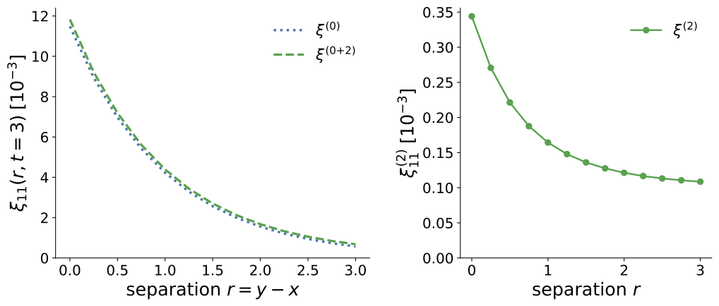
Each order row is one contribution \(\xi^{(n)}\).

The second-order prediction is the partial sum \(\xi^{(0+2)} = \xi^{(0)} + \xi^{(2)}\).

From results/base/orders.csv: \(\xi^{(2)}/\xi^{(0)} = 3.0\%\) at \(r = 0\) and \(19\%\) at \(r = 3\).

Reading the output needs one distinction. Each row labelled with an order is a contribution, xi-n. The prediction at second order is the partial sum: xi-zero plus xi-two.

On the left are the order-zero curve, dotted, and the partial sum, dashed, against separation, in the line styles of the paper. The order-two contribution, on the right, is three percent of order zero at zero separation. It falls off more slowly with separation than order zero, so its share grows to nineteen percent at r equal to three.

The plotting script in the tutorial folder adds the orders explicitly, so the partial sum appears in code rather than being implied by a colour.

Change one physical parameter

sft-wick

1. 01 Formalism
2. 02 Hands-on
3. 03 Non-Gaussian
4. 04 Lensing

Change one physical parameter

configs/01_gaussian.yaml → configs/02_sigma_x_2.yaml

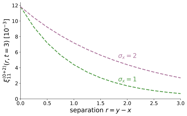
-      spatial:  {type: exponential, sigma_x: 1.0}+      spatial:  {type: exponential, sigma_x: 2.0}⋮-  - {type: table, format: csv, path: results/base/orders.csv}-  - {type: npz, path: results/base/orders.npz}+  - {type: table, format: csv, path: results/sigma_x_2/orders.csv}+  - {type: npz, path: results/sigma_x_2/orders.npz}

$ sft-wick run configs/02_sigma_x_2.yaml

A longer noise correlation length gives longer-range field correlations. The variance at a point is unchanged, so the curves start together.

Now change one physical parameter. Before running, predict the result: a longer noise correlation length sigma-x should give field correlations that extend further.

The second file differs from the first in three lines: sigma-x from one to two, and new output paths, so the first result is kept.

The run takes a few seconds, and the curve does what we expected. Both start at the same value, because the noise variance at a single point has not changed. At separation one the correlation is about sixty percent higher. This is the basic loop of the workflow: one physical scale, one key in the file, one command, one curve.

Checked against 100 000 simulated realisations

sft-wick

1. 01 Formalism
2. 02 Hands-on
3. 03 Non-Gaussian
4. 04 Lensing

Checked against 100 000 simulated realisations

Paper, Fig. 3: \(\xi_{11}\) and \(\xi_{22}\) at \(r = 0.5\,\sigma_x\); lower panels: residual and simulation uncertainty

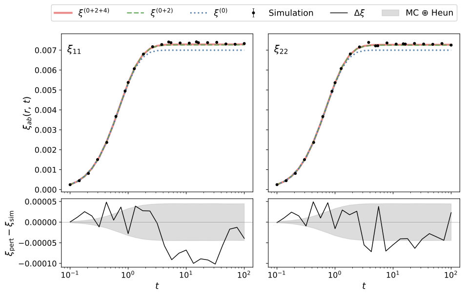
Simulation

Heun integrator with exact coloured noise, \(10^5\) realisations; Monte Carlo error \(\lesssim 0.6\%\).

Expansion

Orders 0, 2, 4. Each even order is smaller than the previous by about \(\lambda = 0.05\).

\(\xi^{(0+2+4)}\) stays within about \(1.5\%\) of the simulation. At late times the residual exceeds the shaded band, most clearly for \(\xi_{11}\).

Does the expansion agree with the stochastic system itself? The paper’s figure compares orders zero, zero plus two, and zero plus two plus four with a direct simulation of the Langevin equations, one hundred thousand realisations, for both diagonal correlators.

The lower panels show the residual and the uncertainty band. Each even order is smaller than the previous one by roughly lambda, five percent. At fourth order the prediction stays within about one and a half percent of the simulation. At late times the residual is larger than the shaded band, most clearly for xi-one-one, so this comparison does not show agreement within every error bar, and the paper does not claim convergence beyond the computed orders.

Non-Gaussian driving

03

Non-Gaussian driving

Back to the opening question: shot noise with the same covariance as a Gaussian drive.

01 · Formalism

02 · Hands-on

03 · Non-Gaussian

04 · Lensing

Part three: non-Gaussian driving.

Shot noise: one parameter sets the non-Gaussianity

sft-wick

1. 01 Formalism
2. 02 Hands-on
3. 03 Non-Gaussian
4. 04 Lensing

Shot noise: one parameter sets the non-Gaussianity

$$\eta_a(x,t) = \sum_k h\,w(x-x_k)\,g(t-s_k) - \vev{\cdot}$$

Poisson events \((x_k, s_k)\) at rate \(\nu\); pulses \(g(\tau) = \Theta(\tau)\,e^{-\tau/\sigma_t}\) and \(w(x) = e^{-|x|/\sigma_x}\).

$$\text{skewness} = \frac{4\sqrt2}{9}\,\frac{1}{\sqrt n},\qquad \text{excess kurtosis} = \frac{1}{2n}$$

\(n \equiv \nu\sigma_t\sigma_x\). Adjusting \(h\) holds the variance \(nh^2/2\) fixed.

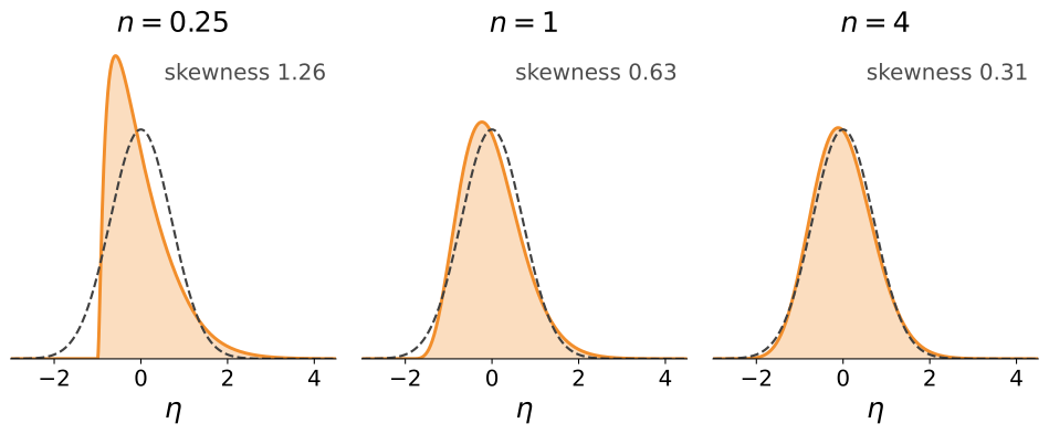
One-point PDF of the drive (orange) and the Gaussian of equal variance (dashed). The worked example and the opening slide use \(n = 1\).

The second worked example keeps the same equations, with the coupling scaled by 0.2, and replaces the Gaussian noise by shot noise. Events arrive at random positions and times with rate nu. Each event starts a pulse that decays exponentially in time and in space, and the mean is subtracted.

Campbell’s theorem gives every cumulant of this noise in closed form. The shape of the one-point distribution depends on one number, n, the mean number of events per correlation cell. Skewness falls as one over root n, excess kurtosis as one over two n. Adjusting the pulse height keeps the variance fixed. So n changes the non-Gaussian part of the noise and leaves the Gaussian part alone.

The worked example uses n equal to one, the middle panel. It is the drive from the opening slide.

Higher cumulants enter as vertices

sft-wick

1. 01 Formalism
2. 02 Hands-on
3. 03 Non-Gaussian
4. 04 Lensing

Higher cumulants enter as vertices

$$\Sint^{\mathrm{K}} = \frac{\ii}{3!}\int\!\dd\bm{z}_1\,\dd\bm{z}_2\,\dd\bm{z}_3\;\cumulant^{(3)}_{abc}(\bm{z}_1,\bm{z}_2,\bm{z}_3)\,\psi_a(\bm{z}_1)\,\psi_b(\bm{z}_2)\,\psi_c(\bm{z}_3) \;-\; \frac{1}{4!}\int\!\cumulant^{(4)}_{abcd}\,\psi_a\psi_b\psi_c\psi_d \;+\;\cdots$$

Counting legs

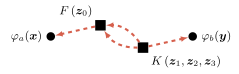
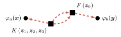
With \(n_F\) cubic vertices and one \(\cumulant^{(m)}\), a diagram of \(\vev{\varphi_a\varphi_b}\) exists only if

$$2 + n_F - m \;\ge\; 0 \ \ \text{and even.}$$

So \(\cumulant^{(m)}\) first enters at order \(m - 1\): \(\cumulant^{(3)}\) at order 2, the FK class.

The two FK diagrams (paper, Fig. 8)

All four propagators are \(\RespOp\). Diagram (b) is (a) with \(\bm{x}\leftrightarrow\bm{y}\).

We met these vertices in part one: response fields only, three for the third cumulant, four for the fourth, with legs at different points.

Which cumulant enters at which order follows from counting legs. A diagram of the two-point function with n-F cubic vertices and one cumulant vertex with m legs exists only if two plus n-F minus m is zero or positive, and even. So the m-th cumulant first enters at order m minus one. The third cumulant enters at order two, together with one F vertex. This is the FK class.

Figure 8 of the paper shows its two diagrams. All four lines are response lines: the third cumulant drives one external field directly, and drives the F vertex through two responses; the F vertex then responds to the other external point. In the package they are contracted by the same engine as local vertices.

xi_12 answers the opening question

sft-wick

1. 01 Formalism
2. 02 Hands-on
3. 03 Non-Gaussian
4. 04 Lensing

\(\xi_{12}\) answers the opening question

$$\xi^{\mathrm{FK}}_{11} = \xi^{\mathrm{FK}}_{22} = 0,\qquad \xi^{\mathrm{FK}}_{12} \neq 0$$

Gaussian theory: symmetric under \((\varphi_2, \psi_2) \to (-\varphi_2, -\psi_2)\). Odd cumulants break it, so Gaussian driving gives \(\xi_{12} = 0\) exactly.

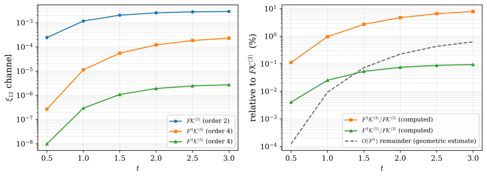
Channel at \(t = 3\)	Order	\(10^{-3}\)
\(F\cumulant^{(3)}\)	2	2.897
\(F^{3}\cumulant^{(3)}\)	4	0.229
\(F^{3}\cumulant^{(5)}\)	4	0.0027
Simulation		\(3.144 \pm 0.032\)

Paper, Fig. 10, coupling amplitude \(s = 0.2\), \(n = 1\)

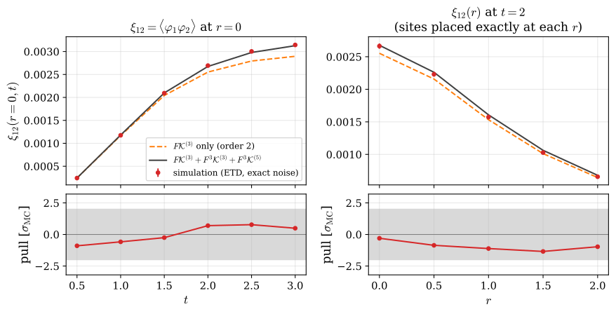
Same covariance, different noise: \(\xi_{12}(t{=}3) \approx 3.1\times10^{-3}\) for shot noise, exactly zero for Gaussian driving.

For this coupling the FK contribution obeys a selection rule. It vanishes for the diagonal correlators xi-one-one and xi-two-two, and survives for the cross-correlator xi-one-two. The reason is a symmetry: with Gaussian noise the theory does not change when phi-two and psi-two change sign together. Odd cumulants break that symmetry.

The dashed line is the FK channel alone; the solid line adds the two order-four channels, F-cubed K-three and F-cubed K-five; the circles are a simulation. At time three the corrections are 7.9 and 0.094 percent of the leading channel, and the simulation agrees within one standard deviation at every time.

This answers the opening question. Two drives with the same covariance give different two-point functions once the dynamics are nonlinear: xi-one-two is about three times ten to the minus three for shot noise, and zero for the Gaussian drive.

More worked examples ship with the package

sft-wick

1. 01 Formalism
2. 02 Hands-on
3. 03 Non-Gaussian
4. 04 Lensing

More worked examples ship with the package

examples/demo2

Deformed Gaussian noise

\(\tilde\eta = \eta + \alpha(\eta^2 - \lambda)\): narrow non-local cumulant kernels, evaluated in \(\RespOp\)-contracted form.

examples/demo4

Asymmetric compound Poisson

One event drives each component with its own amplitude, width and decay.

examples/demo5

White noise, additive and multiplicative

State-dependent noise, against an exact reference.

examples/demo6

Repeated non-local vertices

Two copies of one non-local vertex, \(m = 5\) and \(m = 2\) vertices, a quartic drift next to a cubic one.

examples/demo7

Space, angle and time

Distinct observation points and times; spatial and rotation-invariant angular kernels.

examples/demo8

Beyond exponential response

Time-dependent rates, an oscillator response that changes sign, custom temporal kernels.

Each example compares the package with a reference calculation; see the README in each example folder.

More worked examples ship with the package, each compared with a reference calculation: deformed Gaussian noise with narrow cumulant kernels; one event driving each component differently; additive and multiplicative white noise; repeated non-local vertices and a quartic drift; observables at distinct points, angles and times; and responses beyond the exponential, including an oscillator whose response changes sign.

Weak gravitational lensing

04

Weak gravitational lensing

The application that motivated sft-wick: a light bundle propagating through a random universe.

01 · Formalism

02 · Hands-on

03 · Non-Gaussian

04 · Lensing

Part four: weak gravitational lensing.

A light bundle is a stochastic field

sft-wick

1. 01 Formalism
2. 02 Hands-on
3. 03 Non-Gaussian
4. 04 Lensing

A light bundle is a stochastic field

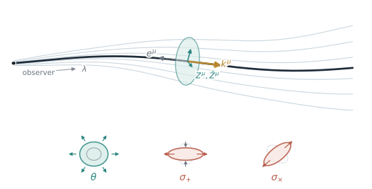
Sachs equations along each ray, with affine parameter \(\lambda\) and sky direction \(\direc\):

$$\begin{aligned}\dot\theta &= -\theta^2 - \sigma_+^2 - \sigma_\times^2 + \Phi_{00}\\ \dot\sigma_+ &= -2\theta\,\sigma_+ + \mathcal{W}_1\\ \dot\sigma_\times &= -2\theta\,\sigma_\times + \mathcal{W}_2\end{aligned}$$

\(\theta\): expansion. \(\sigma_+, \sigma_\times\): shear.
\(\Phi_{00}\): Ricci focusing. \(\mathcal{W}_{1,2}\): Weyl shear, the real and imaginary parts of \(\Psi_0\).

The curvature along the rays is a random field set by the matter distribution.

Lensing paper (Zhang, Bull, Clarkson, Nicola, arXiv:2606.19472): null geodesic congruence and the Sachs scalars

Consider a thin bundle of light rays from a distant source. As it travels, its cross-section expands and is sheared. The Sachs equations describe this along each ray, as a function of the affine parameter lambda. Theta is the expansion; sigma-plus and sigma-cross are the two shear components. The equations are quadratic in these optical scalars, and the curvature drives them: the Ricci term Phi-zero-zero focuses the bundle, and the Weyl terms W-one and W-two shear it.

The curvature along the rays is set by the matter distribution, which we describe statistically. So the light bundle obeys a quadratic stochastic equation, with the same structure as before.

The same equation, with a new dictionary

sft-wick

1. 01 Formalism
2. 02 Hands-on
3. 03 Non-Gaussian
4. 04 Lensing

The same equation, with a new dictionary

sft-wick paper

$$\partial_t\varphi_a = A_{ab}\,\varphi_b + F^{(3)}_{abc}\,\varphi_b\varphi_c + \eta_a$$

Lensing paper

$$\dot{\Dsachs}_a = A_{ab}\,\Dsachs_b + F_{abc}\,\Dsachs_b\Dsachs_c + \Dsrc_a$$

	sft-wick paper	Lensing paper
Field	\(\varphi_a(\bm{x}, t)\)	\(\Dsachs_a(\direc, \lambda) = \sachsvec_a - \sachsvec^{(\mathrm{sa})}_a\), with \(\sachsvec = (\theta, \sigma_+, \sigma_\times)\)
Coordinates	position \(\bm{x}\), time \(t\)	sky direction \(\direc\), affine parameter \(\lambda\)
Driving field	\(\eta_a\)	\(\Dsrc_a = \src_a - \bar{\src}_a\), with \(\src = (\Phi_{00}, \mathcal{W}_1, \mathcal{W}_2)\)
Linear term	\(A_{ab}\)	\(-2\,\delta_{ab}\,\theta^{(\mathrm{sa})}(\lambda)\)
Cumulants	\(\cumulant^{(2)}, \cumulant^{(3)}, \dots\)	linear \(P(k)\), tree-level bispectrum
Observable	\(\vev{\varphi_a\varphi_b}\)	\(\kappa\) and shear correlations: line-of-sight integrals of \(\Dsachs\)

Each column keeps its paper's notation. In the lensing paper \(\varphi\) is the driving field.

Here are the two equations side by side, each in its own paper’s notation. After the mean solution is subtracted, the lensing equation has the same form: a linear term, a quadratic coupling F, and a driving field. The table is the dictionary. The field is the fluctuation of the Sachs scalars, labelled by sky direction and affine parameter. The driving field is the fluctuation of the Ricci and Weyl terms. The cumulants come from a matter model: the linear power spectrum and the tree-level bispectrum. The observables, convergence and shear correlations, are line-of-sight integrals of the field.

One warning about notation: the lensing paper writes phi for the driving field.

Two second-order channels: FF and FK

sft-wick

1. 01 Formalism
2. 02 Hands-on
3. 03 Non-Gaussian
4. 04 Lensing

Two second-order channels: FF and FK

Order-2 diagrams of the Sachs two-point function, drawn by sft-wick (lensing paper)

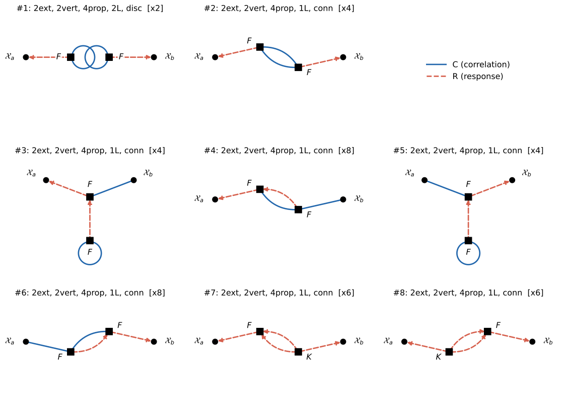
FF, \((n_F, n_K) = (2, 0)\), diagrams #1 to #6

Nonlinear propagation of the bundle. Present for Gaussian curvature too.

FK, \((n_F, n_K) = (1, 1)\), diagrams #7 and #8

The curvature bispectrum enters a two-point function, as \(\cumulant^{(3)}\) entered \(\xi_{12}\) in part 3.

At second order the lensing two-point function has eight diagrams, drawn by sft-wick in the lensing paper. Six have two F vertices: the FF channel. It describes nonlinear propagation of the bundle, and it is present even if the curvature is Gaussian. Two have one F vertex and one K vertex: the FK channel. Here the bispectrum of the curvature enters a two-point function. It is the mechanism we isolated in the shot-noise example, now in cosmology.

On arcminute scales the FK channel exceeds FF

sft-wick

1. 01 Formalism
2. 02 Hands-on
3. 03 Non-Gaussian
4. 04 Lensing

On arcminute scales the FK channel exceeds FF

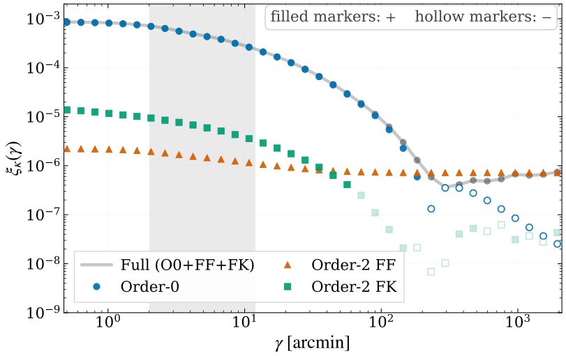
Order 0

The standard linear result; the lensing paper checks it against PyCCL.

At \(\gamma = 0.5'\)

FF / Order-0 \(= 0.3\%\)
FK / Order-0 \(= 1.6\%\)

\(z_s = 5\)Born pathlinear \(P(k)\)tree-level bispectrum\(\ell_{\max} = 15\,360\)

A finite-cutoff worked example, not a calibrated amplitude for the real Universe. Shaded: 2′ to 12′, the range of small-scale cuts in current cosmic-shear analyses.

This is the convergence correlation function for sources at redshift five, split by channel, computed with the package. The grey line is the total. Order zero, in blue, is the standard linear result; the lensing paper checks it against PyCCL. The FF channel is orange and the FK channel green; hollow markers are negative values.

On arcminute scales FK is larger than FF. At half an arcminute, FF is 0.3 percent of order zero and FK is 1.6 percent. These numbers belong to a specific setup: Born paths, the linear matter power spectrum, the tree-level bispectrum, and a finite multipole cutoff. They are a worked example of the method, not a calibrated prediction for the real Universe. The shaded band spans the small-scale cuts of current cosmic-shear analyses, from two to twelve arcminutes.

Summary

sft-wick

1. 01 Formalism
2. 02 Hands-on
3. 03 Non-Gaussian
4. 04 Lensing

Summary

Formalism

Stochastic dynamics → Feynman rules

A response field gives two propagators, \(\CorrOp\) and \(\RespOp\), and vertices for both the nonlinearity \(F\) and the noise cumulants \(\cumulant^{(m)}\).

Software

Diagram table, then numbers

Topology-level contraction, coupling sums and numerical integrals. A YAML file and three commands for a first calculation.

Physics

Nonlinearity mixes statistical orders

Higher noise cumulants reach two-point statistics: \(\xi_{12}\) for shot noise, the FK channel in weak lensing.

$ pip install sft-wick

github.com/StatFieldTheory/sft-wick · tutorial in tutorial/

Z. Zhang, sft-wick, accepted in Computer Physics Communications
Z. Zhang, P. Bull, C. Clarkson, A. Nicola, arXiv:2606.19472

Thank you

ERC, EU Horizon 2020, grant 948764 · RadioForegroundsPlus, HORIZON-CL4-2023-SPACE-01, GA 101135036

To summarise. The formalism: a response field turns a stochastic field equation into Feynman rules, with two propagators and with vertices for both the nonlinearity and the noise cumulants. The software: sft-wick enumerates the diagrams at the level of topologies, routes the component indices, and evaluates the integrals; a YAML file and three commands are enough for a first calculation. The physics: nonlinear dynamics lets higher cumulants of the noise reach two-point statistics. We saw this as xi-one-two in the shot-noise model and as the FK channel in weak lensing.

The package is on PyPI and GitHub, and the tutorial from this talk comes with the recording. Thank you.

Notation used in this talk

sft-wick

1. 01 Formalism
2. 02 Hands-on
3. 03 Non-Gaussian
4. 04 Lensing

BackupNotation used in this talk

Symbol	Meaning
\(\cumulant^{(m)}\)	driving-field cumulant of rank \(m\) (\(m\) legs); \(\kappa\) is reserved for the lensing convergence
order \(n\)	number of vertices (\(F\) or \(\cumulant\)) in a diagram; \(F^{3}\cumulant^{(3)}\) is order 4
\(\xi^{(n)}\), \(\xi^{(0+2)}\)	contribution at order \(n\); partial sum of orders 0 and 2
\(\varphi_1, \varphi_2\)	components as in the paper; YAML arrays use indices 0 and 1
Itô	\(\Theta(0) = 0\); a Stratonovich model must be converted first
n_samples	quasi-Monte Carlo points per diagram integral, not stochastic trajectories

Backup: the notation used in the talk.

First-order diagrams of a three-point function

sft-wick

1. 01 Formalism
2. 02 Hands-on
3. 03 Non-Gaussian
4. 04 Lensing

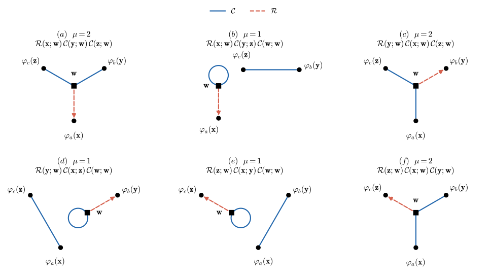
BackupFirst-order diagrams of a three-point function

Paper, Fig. 12. Of 15 Wick pairings, 6 vanish under Itô; the other 9 group into these 6 topologies.

Backup: the six first-order diagrams of the three-point function, the first row of Table 2.

Shot-noise example, channel by channel

sft-wick

1. 01 Formalism
2. 02 Hands-on
3. 03 Non-Gaussian
4. 04 Lensing

BackupShot-noise example, channel by channel

Paper, Fig. 11: the three computed channels of \(\xi_{12}\), and the corrections relative to \(F\cumulant^{(3)}\)

Backup: the computed channels of xi-one-two against time, and the size of the order-four corrections.

Lensing FK channel and the multipole cutoff

sft-wick

1. 01 Formalism
2. 02 Hands-on
3. 03 Non-Gaussian
4. 04 Lensing

BackupLensing FK channel and the multipole cutoff

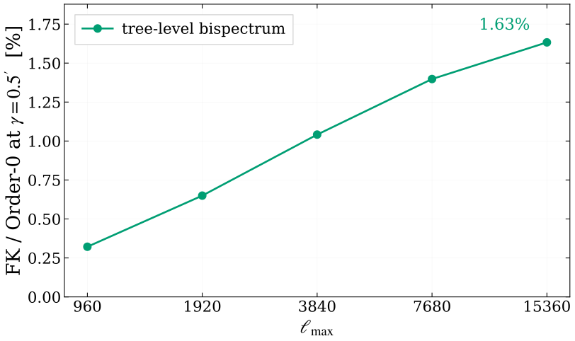
Tree-level bispectrum, \(z_s = 5\), \(\gamma = 0.5'\). Replotted from the frozen corrected products; the PDF figure in the current lensing manuscript shows an earlier value.

Backup: the FK channel at half an arcminute against the multipole cutoff, from the frozen corrected products. It still grows at the largest cutoff, so the value on the main slide is a finite-cutoff number.