Part 3 · Model → plan → inference
Designing a sampler for the model
BlackJAX · NumPyro Powerful sampling
One model: field + nonlinear shape + gain + noise
BLOCKS Which parameters
METHODS What can be sampled
PROPOSALS How do we make the
For each large model, we engineer the Gibbs plan again. Months of bespoke work before the first useful chain.
Bayesmith Analyse the model. Compile its sampling plan.
Reusable design, before sampling.
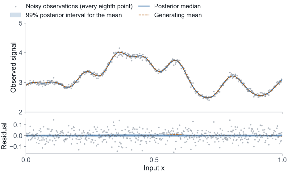
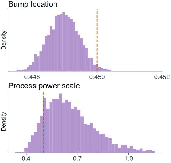
The previous examples share a design problem. BlackJAX and NumPyro already offer powerful sampling and posterior analysis. This saved model combines a random field, nonlinear response, background, gain and signal-dependent noise. Before running it, someone must decide which parameters move together, which conditionals can be solved directly, and where useful proposals are needed. For very large scientific models, in my experience this becomes months or years of bespoke work. [Advance.] I designed Bayesmith to make that work reusable. It analyses the declared model before sampling and compiles supported blocks and update strategies. The numerical backend then executes those updates. [If asked.] Development time is personal experience, not an industry measurement. The figure is the saved composed-process synthetic example. Bayesmith adds structural planning rather than replacing numerical backends; demonstrated execution uses NumPyro. BlackJAX is ecosystem context, not an implemented adapter claim. The planner does not promise an optimal Gibbs scheme or convergence for every DAG.
Part 3 · Model → plan → inference
Model structure guides the sampling strategy
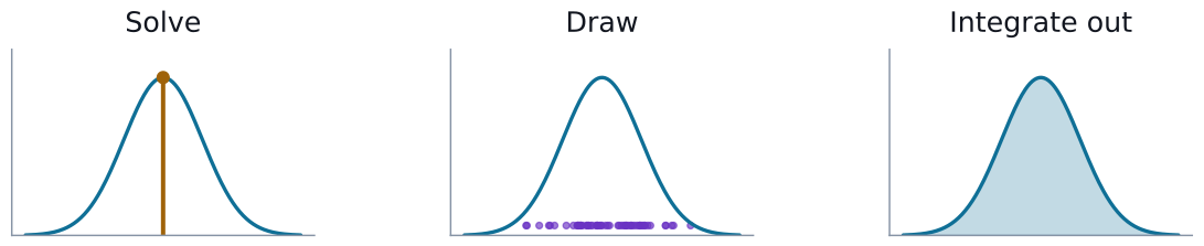
Draw a whole field. Gaussian constrained realisationsOne update, all coordinates.
For a Gaussian full conditional.
Change coordinates. Products become sums.
Exact log-space GCR needs a Gaussian log-data law.
Sample less. Integrate out a compatible
Retain its uncertainty and normalisation.
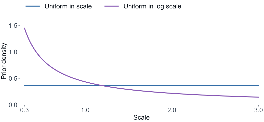
Make priors explicit. A “flat” prior depends
Inspect the choice. Keep the declared prior.
Let the graph form the blocks. Field + background
Shape + gain + power + noise
Actual generated plan · update each block conditional on the other.
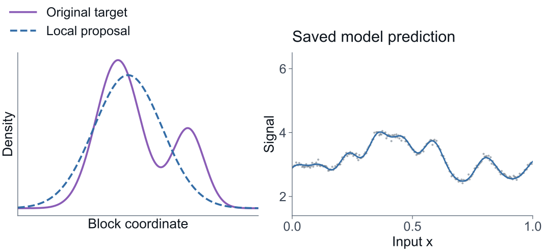
Propose an easier move. GLS · log-linearCorrect against the original target.
MH retains the model, priors and support.
Whole-field draws Gaussian conditionals
Log-space structure Products → linear form
Analytic collapse Fewer sampled variables
Prior analysis Explicit choices
Automatic blocking A model → a sweep
Structured proposals Easier moves + correction
One model. A reusable sampling plan.
Field draws
Log space
Collapse
Priors
Blocks
Proposals
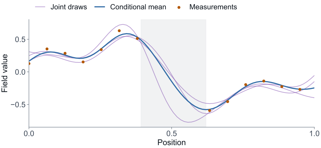
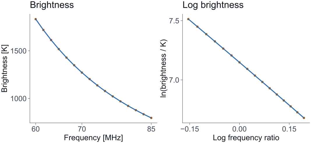
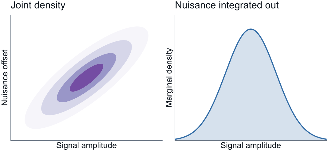
A Gaussian conditional lets us draw an entire field together, including the uncertainty in missing data. [Advance.] Under a Gaussian log-data law, logarithms expose another linear problem: products become sums, and we can draw in those coordinates. [Advance.] Some nuisance blocks can be integrated out, leaving fewer variables to sample while retaining their uncertainty. [Advance.] Prior analysis makes the choices explicit. Uniform in scale and uniform in log scale describe different beliefs; the declared prior is preserved. [Advance.] Here is an actual traced model and its returned sweep: field and background in a corrected proposal block; the nonlinear and hyperparameter remainder in NumPyro. [Advance.] Structured proposals exploit an easier solve, then MH checks the original target. [Advance.] These are reusable moves selected from the model’s structure. [If asked.] The Gaussian field, marginalisation, two prior curves and target/proposal densities are analytic teaching illustrations of the supported method laws, not additional package benchmark runs. Log spectra, observed signal, predicted mean and block plan are saved synthetic examples. GCR needs the full conditional, positive precision and compatible support. Logging arbitrary additive-Gaussian data is not an exact log-space route. The log-spectra panel uses the adopted Gaussian log-space survey model; its physical qualifications are retained in the later map demo. Analytic elimination is limited to supported integrable blocks and preserves determinant terms. The prior comparison does not claim automatic prior substitution; conditional Jeffreys/Fisher tools expose coordinate and local information questions. The composed case uses bounded priors and signal-dependent noise, hence corrected proposals plus NUTS rather than untruncated GCR. All factors and forward/reverse proposal densities remain in MH. Correct target invariance alone is not finite-chain convergence or a guarantee of optimal performance. Details and saved diagnostics are in backup.
Part 3 · Model → plan → inference
Sky and instrument in one model
Bayesmith
Rheplicant
A DAG is a Bayesian model. an observation.
The same graph language, carried into the observing system.
Bayesmith: a DAG is a Bayesian model. [Advance.] Rheplicant: a DAG is an observation. The graph language stays; what we compose changes. Add uncertain parameters, priors and a likelihood around that observing system, and we have the model Bayesmith can analyse. [If asked.] Conceptual bridge, not a guarantee that every observation DAG has an eligible or efficient Gibbs plan. This single reversible build changes the tool and the object together; review and print show the final Rheplicant state.
Part 3 · Model → plan → inference
RHINO observation and inference
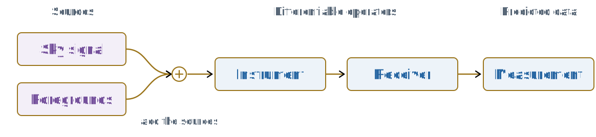
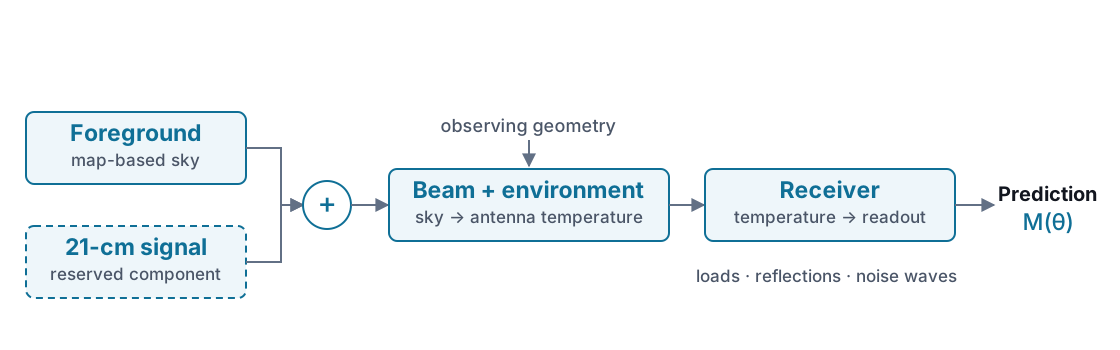
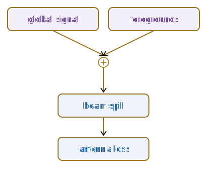
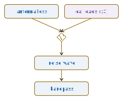
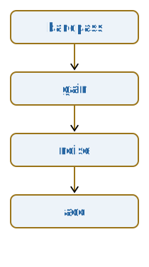
Once the observation is an executable model, its structure can also guide the inference. Rheplicant composes the data model from differentiable operators: sources combine, then pass through the instrument and receiver into measurements. This is the same graph language we have just seen. [Advance.] Add uncertain parameters, priors and a likelihood, and Bayesmith can analyse the Bayesian model. It groups compatible parameters and chooses supported updates; the numerical backend executes the sampling plan. The scientist declares the physics, and the machinery makes the inference design reusable. For RHINO, this is the connection between a sky description, an instrument response, and inference over uncertain parameters. Next I will show the same inference idea in a synthetic sky survey. [If asked.] This is a grouped overview of the existing native radio-tour assembly, not a new run or a literal Gibbs block assignment. Instrument and receiver boxes contain multiple physical operators; the calibration branches are omitted from this overview. No arbitrary DAG, optimal strategy or general convergence is promised. The following two pages show saved whole-map posterior draws in a synthetic narrow-beam survey. Scale examples, agent tool records and campaign information remain in the backup menu.
Part 3 · Bayesian sky inference
A synthetic sky and its observation
Joint inference Brightness · spectral shapeAll positions together
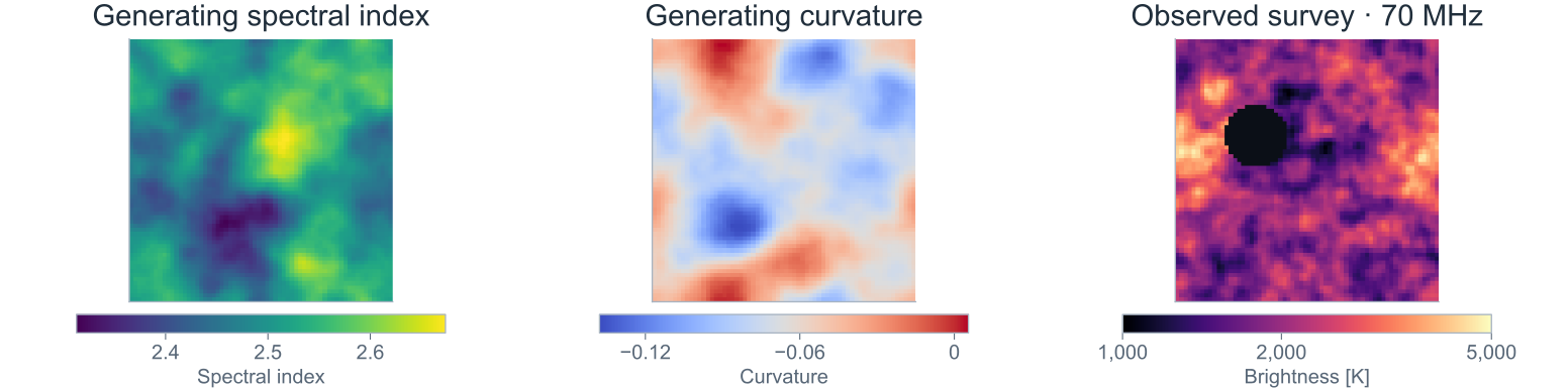
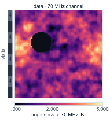
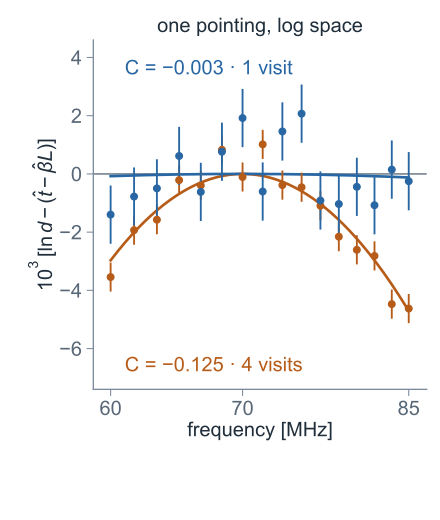
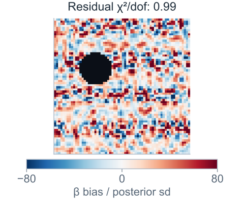
This is a synthetic narrow-beam survey, not a resolved RHINO observation. It illustrates a reusable inference method with an adopted curved-power-law sky model. It does not claim that the SyncMoments model is already integrated into this pipeline. Let me turn the observation model into a concrete example. The spectral index tells us how steeply brightness falls with frequency; spectral curvature tells us how that slope changes. Both vary across this synthetic sky. Rheplicant produces the simulated observation on the right, including a patch with no data. [Advance.] These two example spectra belong to that same survey. We infer the brightness and spectral shape at all positions together, using their shared spatial structure. Bayesmith supplies the Gaussian field update for the adopted log-space model. The model connects an observing system to a whole-field inference problem. [If asked.] The displayed source fields are point values on the pointing grid; the inferred maps are beam moments, with the mixture contribution to curvature included. The beam is 1.5 degrees and achromatic in the main case; spatial fields are smooth on that scale. The saved forward calculation used Pipeline(SkySourceOperator(sky_model=MapSky, projector=MatrixProjector)); radiometer noise and hit masks were added by the demo code, not by a displayed receiver assembly. The curves on the spectrum plot are posterior mean curvature contributions, not an independent polynomial fit. [From twin to resolved sky.] Give the sky box in the observation-model overview a spectral index and a curvature in every direction. RHINO's forty-degree beam cannot resolve those maps; a narrow-beam survey can. So I simulate one with rheplicant: a sky four times finer than the pointings, a curved power law in every pixel, a beam of 1.5 pointings, noise of one part in a thousand per channel, and one unobserved hole. [Advance.] The inference model takes the log of each pointing's spectrum. The noise becomes additive and the curved power law a quadratic in L. On the right, two pointings with the fitted power law removed. [Advance.] Gaussian-field priors on β and C make it one linear-Gaussian block of 12,288 unknowns, which bayesmith draws from exactly. [Advance.] Why maps: one global β and C gives χ² per degree of freedom of 123; β and C per pointing give 0.99. [If asked.] The sky box is the graph's map-based foreground. The simulator applies the beam in temperature; the noise is radiometer noise for one visit, and four visits halve it. The log turns multiplicative noise into additive noise of width f, after a known shift of f squared over two. f = 10⁻³ is a 0.64 s visit in 1.56 MHz channels. The two pointings follow a fixed rule: the four-visit pointing with the largest posterior-mean |C| and the one-visit pointing with the smallest; their error bars are in log space. The prior describes the beam-smoothed field, the field the data measure. bayesmith's factor_partition finds the log block; compile() does not choose that route for this graph yet, so the draws call log_linear_operator and a jitted gcr_sample. The route table is in backup.
Part 3 · rheplicant + bayesmith · Synthetic narrow-beam survey · Posterior maps
One posterior draw is a whole sky
Joint sky maps · independent draws · uncertainty follows coverage
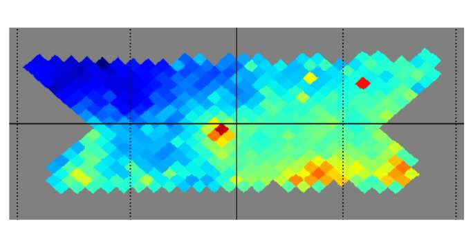
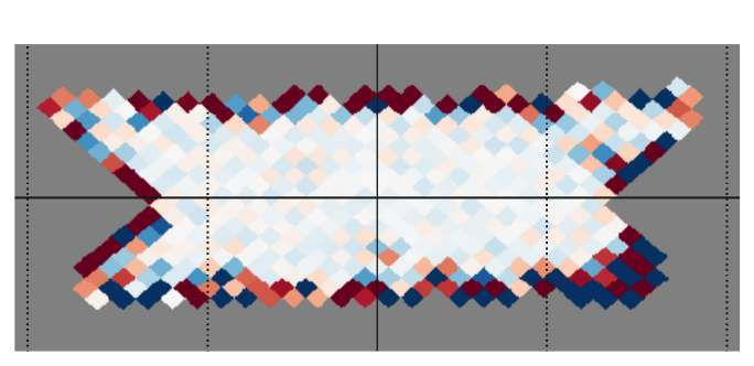
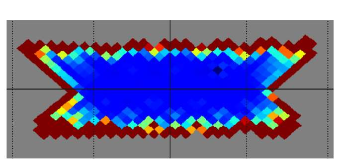
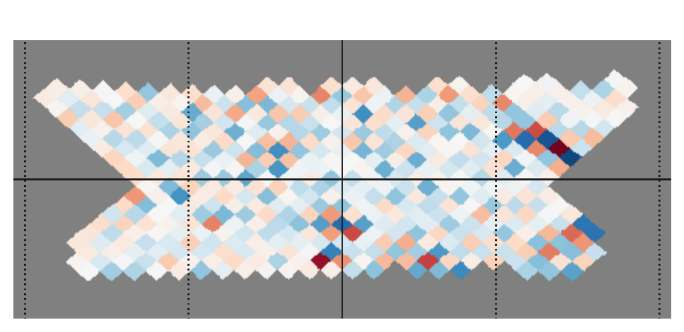
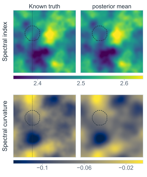
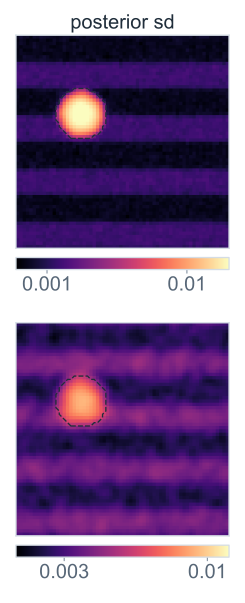
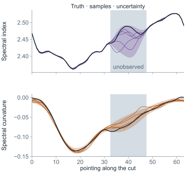
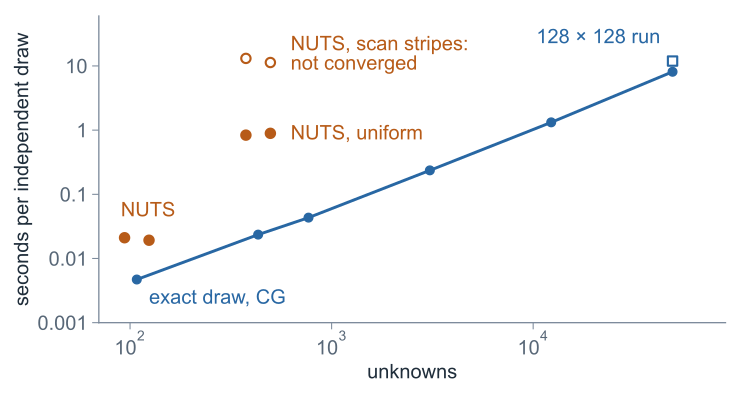
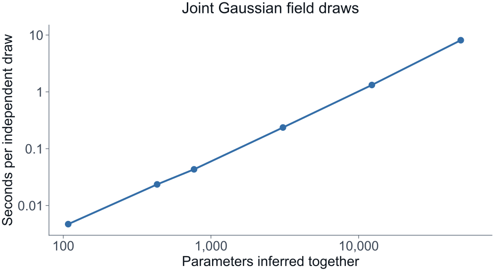
This is a synthetic narrow-beam survey, not a resolved RHINO observation. It illustrates a reusable inference method with an adopted curved-power-law sky model. It does not claim that the SyncMoments model is already integrated into this pipeline. The top row is spectral index: how steeply brightness falls with frequency. The bottom row is spectral curvature: how the slope changes. We compare the known truth with the posterior mean. [Advance.] The uncertainty follows the observing coverage; it increases in the missing patch. [Advance.] These coloured curves are independent posterior draws through that patch. Each draw contains a complete, spatially correlated sky. [Advance.] This is the capability to remember: whole maps and their joint uncertainty, including the places where data are missing. [If asked; technical details.] [Let the maps sit.] Top row the spectral index at 70 MHz, bottom row the curvature; left the truth, right the posterior mean. The truth is the beam average the data measure; the physical checks are in the physical/model-check backup. [Advance.] The posterior standard deviation follows the scan: stripes where it passed once or four times, and the hole, where only the neighbours and the prior constrain the map. [Advance.] A cut through the hole: the truth in white, five independent posterior draws, and the two-sigma band from 200 draws. Outside the hole the draws sit on the truth; inside they spread. Each draw is a whole map of 12,288 numbers. [Advance.] A draw takes 1.3 seconds and does not depend on the previous one: no chain and no burn-in. Its solver error is certified below a hundredth of a posterior standard deviation in every pixel. At 432 unknowns with the same scan pattern an exact draw takes 23 milliseconds. NUTS took 3 minutes per chain for a thousand draws after a thousand warm-up steps and had not converged: the two chains disagree, R-hat up to 1.092 for a β pixel, and one chain has as few as 14 effective draws for a curvature pixel. 12,288 sits on the parameter-count ladder, between the drift scan and the 21-cm cube. [If asked.] The truth is weighted by the sky brightness. For β the posterior sd is about 1.2 × 10⁻³ in single-visit stripes, 7.4 × 10⁻⁴ in four-visit stripes and 1.0 × 10⁻² in the hole. Where NUTS converged, its posterior means differ from the exact draws by at most 0.12 NUTS standard deviations in uniform coverage at 432 unknowns (two chains, R-hat at most 1.01) and by at most 0.15 at 108 unknowns (means and sds pooled over two chains, R-hat at most 1.01, at least 983 effective draws per chain). In the stripes 82 of the 144 curvature pixels have R-hat above 1.01. The NUTS cost per effective draw is the wall time of one chain, compilation and warm-up included, over its smallest effective sample size among the β and C pixels: 0.84–0.89 seconds in uniform coverage, and 11–13 seconds in the scan stripes, where the effective sample sizes come from unconverged chains. NUTS was not run at 12,288. At this size a dense Cholesky factorisation, with t eliminated pointing by pointing, also draws exactly: 1.5 seconds to build, factorise and solve for the mean, then 0.3 milliseconds per draw, so here it is faster for more than one draw. It is the check in the backup. Its memory grows as the square of the number of unknowns and its cost as the cube; the conjugate-gradient route needs only applications of the operator. The solver bound uses the residual and the prior: in whitened coordinates the posterior precision is at least the identity, so the residual norm bounds the error of every pixel in units of its posterior standard deviation. The relative error of the whole vector is certified below 5.0 × 10⁻⁴, with the largest eigenvalue bounded analytically; bayesmith's default twelve-step estimate of that eigenvalue is 0.6 per cent low on this operator. Per pixel, the data alone fix C only to 0.025, about the rms of the C field itself (0.025). The joint posterior reaches 0.0036 in single-visit stripes because the smoothness prior shares information between pixels, so the curvature map leans on the prior; the physical/model-check backup shows what a wrong prior does. The cut was fixed through the hole centre before plotting. Along it the curvature truth leaves the two-sigma band at 3 of 64 pointings, 1 of them in the hole; over 16 realisations the 68 per cent intervals in the hole cover 66% (β) and 71% (C). Timings were taken on an Apple M3 Ultra with other jobs running (one-minute load 2.1 to 8.4); the NUTS chains were rerun one at a time, at load 1.8 to 3.2.
Discussion · Technical backup
Choose a layer to open
Part 1 · Lensing Part 2 · Synchrotron
Use this page as a navigation menu during questions. Each backup opens a specific issue rather than restarting the talk.
Backup · Part 1 · The toy model
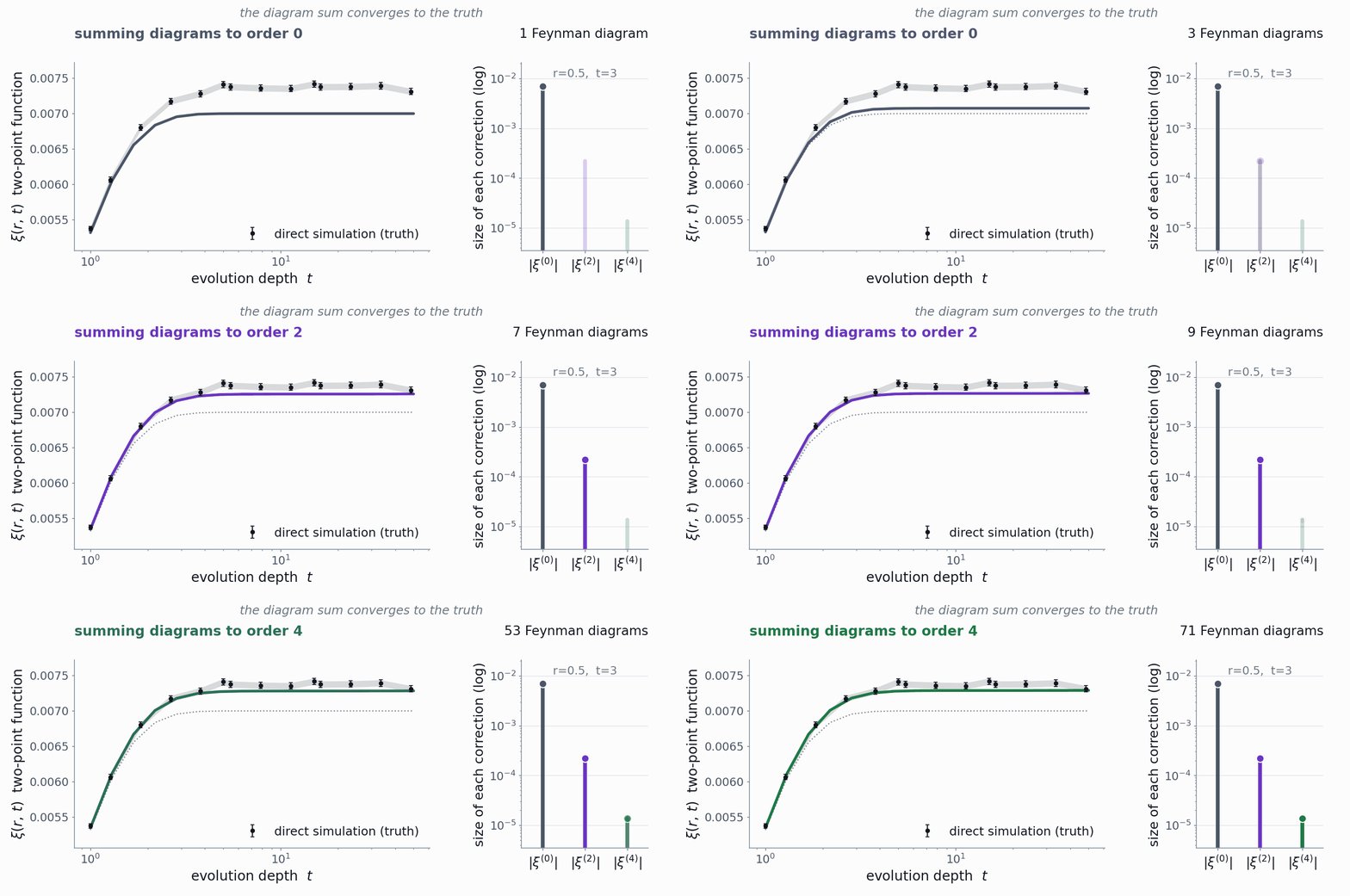
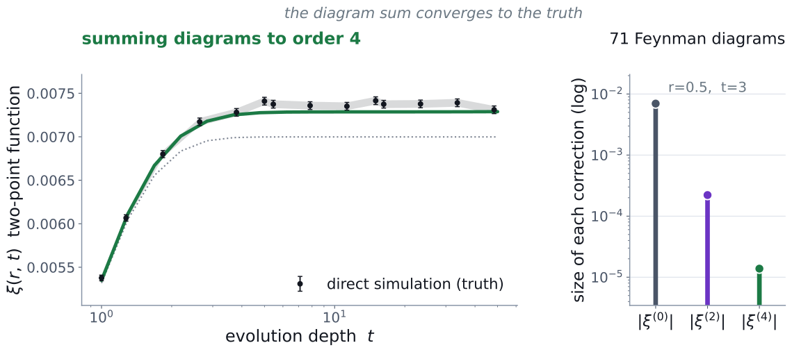
Gaussian baseline: the diagram sum approaches the simulation
\[\dot\phi_a=-\gamma\,\phi_a+s\,F_{abc}\,\phi_b\phi_c+\eta_a\]
Two coupled fields on a line: the same shape as the Sachs system, but small enough to integrate directly. For now the drive \(\eta\) is Gaussian : \(\mathcal K^{(n)}=0\) for \(n\ge3\), so there are no cumulant vertices.
Each order brings the sum closer to the simulation. At order 4 the simulation still lies above it at 12 of 14 times, by up to 3.0 Monte-Carlo error bars. A Gaussian drive cannot show the effect we are after.
[Let the animation run once. Do not talk over the whole thing.] First the check you have to do. Take a toy with the right structure: two coupled fields, a quadratic vertex, a random drive, but ordinary Gaussian noise, so only the dynamical nonlinearity is in play. Compute order zero, add order two, add order four, and compare with a brute-force Langevin simulation of the same equation. Each order moves the sum toward the simulation: the rms offset falls from 7.2 to 2.1 to 1.7 error bars. At order four the simulation still lies above the sum at 12 of the 14 times, by up to 3.0 error bars. This test cannot see the cumulant vertices: Gaussian noise has none, so nothing here probes K. For that we need a drive with the same power spectrum and different statistics. [If asked: the simulation has 10⁵ Langevin realisations at time step 0.02; the error bar is the Gaussian estimate, the square root of ξ(0)² + ξ(r)² over N. The diagram integrals use Gauss–Legendre quadrature with 20 nodes per dimension; 28 nodes move the order-four sum by at most 0.04 error bars, so the quadrature is not the cause of the offset. Other causes have not been tested.]
Backup · Part 1 · The toy model
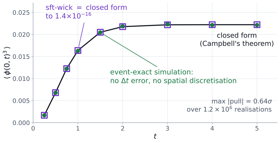
Where truth is known, we hit it exactly
\(1.4\times10^{-16}\)
sft-wick vs closed form
0.64 σ
vs an event-exact simulation, 1.2×10⁶ realisations
[Two things to land here, and only two.] Turn the quadratic coupling off for a moment. The series then terminates: the m-point function is exactly one diagram, one cumulant vertex with m response legs, and nothing can mix into it. So there is a closed form, and I can ask whether the code reproduces it. It does, to one part in ten to the sixteen. That is machine precision; there is no approximation left to measure. Second, the reference simulation has no discretisation error of any kind: the response to one exponential pulse is analytic, so events are summed exactly. Agreement at zero point six sigma over more than a million realisations. That is the exact tier. Now turn the coupling back on.
Backup · Propagation variables
Jacobi and Sachs describe the same propagation
Jacobi map \(D\) \[D''=\mathcal T D\]
linear in \(D\), random multiplicative tidal matrix; angular separation at the observer → transverse separation at the source
Optical rates \(S\) \[S'+S^2=\mathcal T\]
Riccati form: additive forcing, quadratic drift; the Sachs scalars are the components of \(S\)
\[S=D'D^{-1},\qquad \mathcal A=D/\bar D,\qquad \mu=(\det\mathcal A)^{-1}\]
A rate integral recovers the matrix map only through ordered evolution; magnification and reduced shear are readouts of \(\mathcal A\), not of \(\int S\).
The Jacobi map is linear in D with a random multiplicative tidal matrix. The Sachs or Riccati representation evolves the rate matrix S with additive forcing and a quadratic drift; its components are the optical scalars used in the main talk. They describe the same propagation on their shared domain. Recovering the Jacobi map from rates needs ordered evolution; magnification and reduced shear are readouts of the normalised map, which is why the main two-point number is the linear-order kappa, minus the integral of delta-theta, rather than the full Jacobi convergence. The Riccati form holds away from the observer vertex and before caustics.
Backup · Optical readout
Rates, maps and image observables differ beyond leading order
\[\mathcal A=(1-\kappa_A)I-\gamma_+\sigma_3-\gamma_\times\sigma_1+\omega\epsilon\]
\[g=\frac{\gamma}{1-\kappa_A},\qquad \mu=(\det\mathcal A)^{-1}\]
\[\kappa=-\int_0^{\lambda_s}\delta\theta\,d\lambda,\qquad \kappa_{\ln}=-\ln(D_A/D_0)\]
The two-point slides compute \(\langle\kappa\kappa\rangle\) with this \(\kappa\), the paper's linear-order convergence. Beyond linear order the same integral equals \(\tfrac12\ln\mu\) at fixed affine endpoint on the positive-parity branch and differs from \(\kappa_A\). All of these coincide at leading order and differ beyond it.
The normalised Jacobi map decomposes into trace convergence kappa-A, shear and rotation. Reduced shear is a ratio and magnification is a determinant. The kappa of the main slides is minus the integral of delta-theta, the paper's linear-order convergence: the Sachs evolution is kept nonlinear and the conversion to observables is linearized. Beyond linear order the same integral is one half log mu at fixed affine endpoint on the positive-parity branch, which differs from kappa-A. The toy's kappa-ln is a log-distance ratio. These definitions coincide at leading order and should not be conflated beyond it. The two-point example folds the correlation of that kappa and includes neither the external map insertions nor a galaxy estimator; the PDF toy histograms kappa-ln. Beyond leading order neither is identified with kappa-A or with g.
Backup · Response construction
The auxiliary field enforces the optical equation
\[1=\int\mathcal D\mathcal X\;\delta\big[f[\mathcal X]-\textcolor{#2867a3}{\varphi}\big]\,\mathcal J,\quad f=\dot{\mathcal X}-A\mathcal X-\textcolor{#b75b18}{F\mathcal X\mathcal X},\quad \mathcal J=\mathrm{Det}\,\frac{\delta f}{\delta\mathcal X}\]
\[\delta(r)=\int\!\frac{d\widetilde{\mathcal X}}{2\pi}\,e^{-i\widetilde{\mathcal X}r},\qquad \textcolor{#2867a3}{W[J]}=\sum_{n\geq2}\frac{1}{n!}\int \mathcal K^{(n)}(1,\ldots,n)\,J_1\cdots J_n\]
\[S=i\!\int\!\widetilde{\mathcal X}(\dot{\mathcal X}-A\mathcal X-\textcolor{#b75b18}{F\mathcal X\mathcal X})-\textcolor{#2867a3}{W[i\widetilde{\mathcal X}]}\]
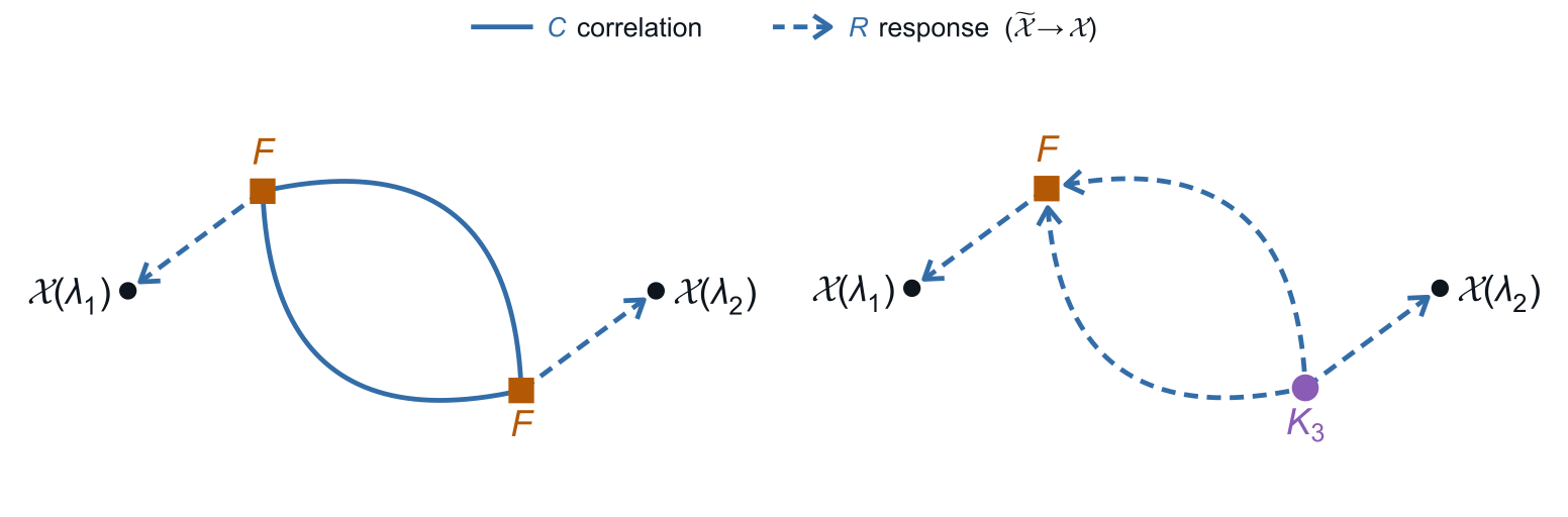
\[\langle\mathcal X\widetilde{\mathcal X}\rangle_0=-iR,\quad\langle\mathcal X\mathcal X\rangle_0=R\mathcal K^{(2)}R^{\mathsf T},\quad\langle\widetilde{\mathcal X}\widetilde{\mathcal X}\rangle_0=0\]
Fixed initial state at the observer; mean driver matched to the background. Pre-point (Itô) slicing: the Jacobian \(\mathcal J\) is field-independent, and in the time-sliced form it is 1, so \(\langle1\rangle=1\).
The functional delta restricts the optical history to the equation driven by the curvature. Its Jacobian depends on the discretisation prescription; for the fixed-initial-state pre-point Itô slicing used here it is field independent, and in the time-sliced form it equals one, so the normalisation is one. Fourier representation of the delta introduces the response field. Averaging the driver gives its cumulant functional evaluated at i times the response field. The mixed Gaussian propagator is minus i times the causal response, the physical covariance is R, script-K two, R transpose, and there is no response-response contraction. Convention: R(λ, λ′) vanishes for λ ≤ λ′, and expectations are normalised.
Backup · Counting conventions
Several independent order counts, and a one-line mixing identity
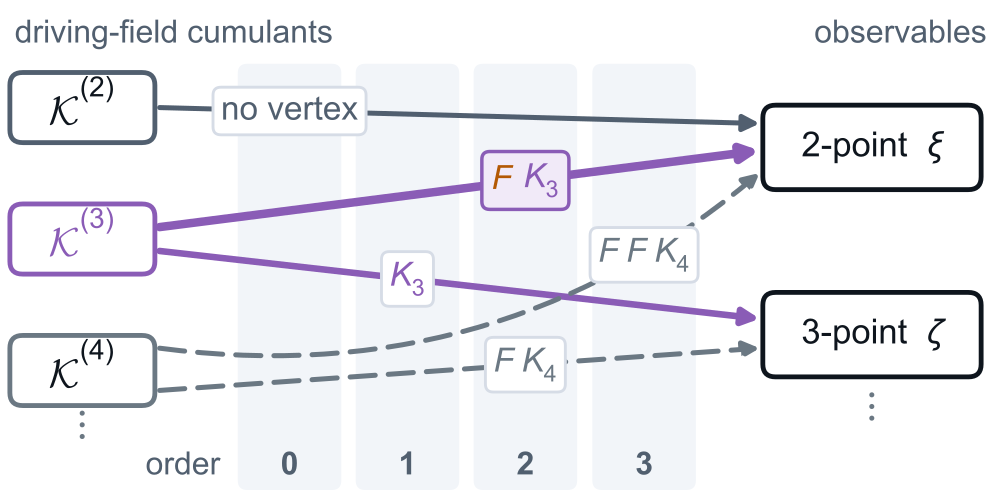
Count Example Matter perturbations linear \(P\), tree-level \(B\) from gravity Driver cumulants \(\mathcal K^{(2)},\mathcal K^{(3)},\mathcal K^{(4)},\ldots\) Optical insertions \(FF\), \(FK_3\), \(F^3K_3\), \(F^3K_5\) Source-field order \(\gamma^{(1)},\gamma^{(2)},\ldots\) in the readout
Why a two-point output reads higher input statistics, in one line: take a centred unit-variance \(X\) with cumulants \(c_3,c_4\) and a quadratic response \(Y=X+a(X^2-1)\).
Exact for the polynomial map; a toy for the structure, not an optical coefficient.
\[\mathrm{Var}\,Y=1+\underbrace{2a\,c_3+a^2c_4}_{\text{non-Gaussian driver}}+\underbrace{2a^2}_{\text{Gaussian, nonlinear}}\]
Order means different things in these layers. A tree bispectrum is built beyond a Gaussian linear seed even when the power spectrum is kept linear. The driver cumulant rank says how many driver fields connect. The optical insertion count says how many Sachs vertices occur. The source-field order counts powers in the external readout. The one-line identity on the right shows the structure: the variance of a quadratic response contains the third and fourth cumulants of the input and a purely Gaussian nonlinear term. It is a polynomial toy, not an optical coefficient. Second-order perturbation theory does not fix these counts, and a single topology is not a complete order.
Backup · The toy model
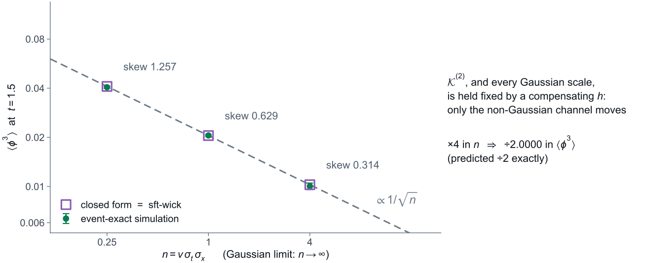
One dial moves the non-Gaussianity and nothing else
The model has one dimensionless number: the mean number of events per correlation volume. Everything about the non-Gaussianity is controlled by it, skewness like one over root n and excess kurtosis like one over n, while the event amplitude compensates to keep the variance fixed. Sweeping it moves the non-Gaussian channels and nothing else. Closed form, sft-wick and the event-exact simulation agree at every point. Residuals are within 0.8 sigma at n = 0.25, 1 and 4.
Backup · The toy model
What is computed, and what is left
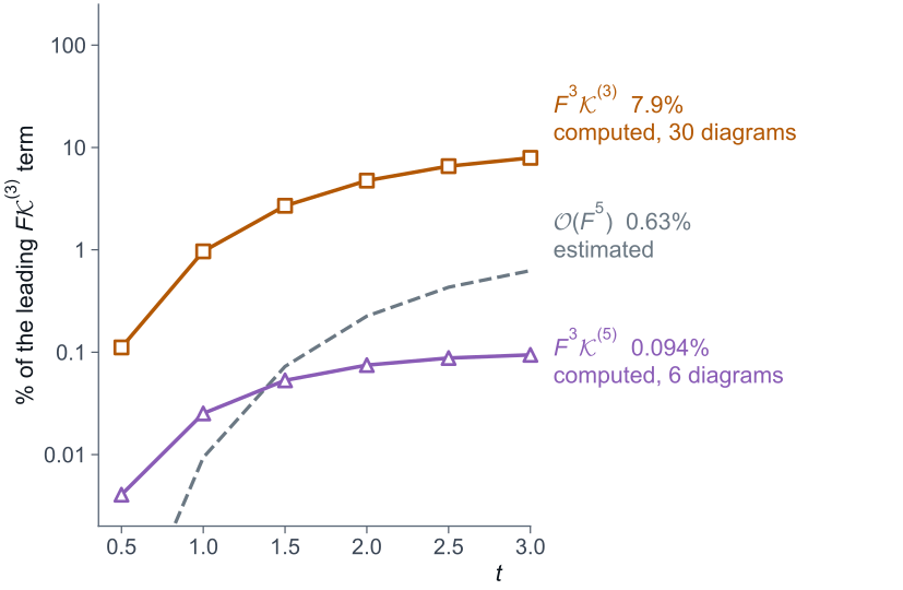
The \(\mathcal K^{(5)}\) ladder is computed: 0.09% of the leading channel at \(t=3\).
Not computed: \(F^4\mathcal K^{(3)}\mathcal K^{(3)}\), the next order the selection rule and the symmetry allow, and \(\mathcal O(F^5)\), estimated geometrically at 0.6% at \(t=3\).
The three-point check at \(F=0\) and the two-point leak test the expansion, the enumeration and the evaluation. They do not test the lensing vertex table, the Limber reduction, the cutoff or the bispectrum model.
[Backup; what is computed and what is left.] The computed channels are on a log axis, as a per cent of the leading F script-K three term at each time. The five-point cumulant ladder is computed: nine hundredths of a per cent at t equals 3. Two pieces are not computed. The fourth order with two three-cumulants, one for each of the two independent drives, is allowed by the selection rule and by the symmetry. The fifth order in the coupling is estimated geometrically, as the square of the computed third-order ratio: 0.6 per cent at t equals 3. The toy tests the machinery, not the cosmological inputs. [If asked: the saved two-point simulation uses six seeds × 400,000 realisations per seed, 2,400,000 in total.]
Backup · Two-point scope
The saved FF/FK calculation has a precise boundary
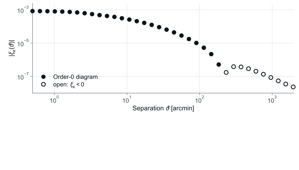
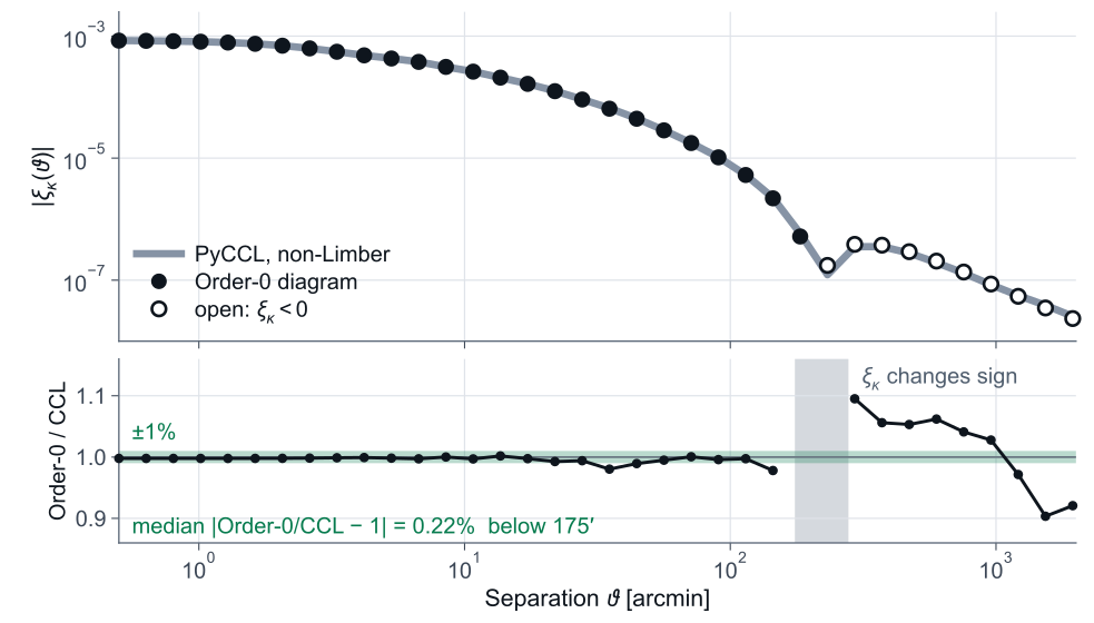
Statistic raw \(\langle\kappa_1\kappa_2\rangle\) and \(\xi_+\), \(\kappa=-\int\delta\theta\,d\lambda\) at linear order; FF includes an induced-mean product Path & reference Born-path Sachs sector, fixed affine endpoint 2313.03 Mpc; nominal \(z_s=5\) Input linear \(P\), tree-level \(B\); Limber equal-shell \(\mathcal K^{(3)}\); vertex cutoff 15360 FK / Order-0, \(\xi_\kappa\) 1.79% (0.5′) · 1.46% (2.06′) · 1.47% (5.30′) · 1.43% (10.77′) · 1.42% (27.7′) · 1.28% (56.3′) FK / Order-0, \(\xi_+\) 1.08% · 0.71% · 0.56% · 0.44% · 0.34% · 0.31% Code sft-wick pinned at a4befdc with the nonlocal-coupling leg-order fix; anchors reproduced at rtol \(10^{-12}\)
These details define the scope of the quantitative result. It is a raw moment of kappa, minus the integral of delta-theta, on a Born path at a fixed affine endpoint, with linear power and a tree bispectrum. The six saved angular nodes and both ratios are listed; the main slide shades the two-to-eleven arcminute interval. The fold uses the pinned sft-wick commit with the leg-order fix, and the plotted anchors reproduce the saved arrays to one part in ten to the twelve. The numbers are replotted from saved products; there is no new cosmological fold, cutoff sweep or survey forecast.
Backup · How solid
UV sensitivity of the collapsed configuration, and a Monte-Carlo check of the fold
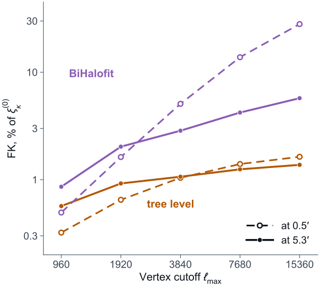
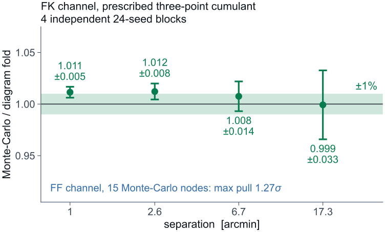
post-fix cutoff ladder (5 Oct), a separate product direct Monte Carlo of the Sachs equation vs the diagram fold Left: a collapsed configuration is a coincident-point moment, so it is UV-sensitive by construction. This is the cutoff ladder of 5 October, the panel of slide 21: FK as a per cent of Order-0 for the convergence correlation against the vertex cutoff, dashed at half an arcminute, solid at 5.3. At tree level the last doubling adds 17 per cent at half an arcminute and about 9 to 11 per cent in the 2 to 11 arcminute band. With BiHalofit it adds 103 per cent at half an arcminute and 25 to 38 per cent in the band; that sum has not converged by ell max 15360, so no cutoff-independent nonlinear amplitude is quoted, and the 5 to 10 per cent of slide 21 is the value at ell max 15360, still rising. The ladder is a separate product from the 12 September fold of slide 20, accepted for finite amplitudes and sampled signs only, not as a scientific result: it sits at the true redshift-5 plane, uses the vertex tables with the 3 October spin-2 sign correction and sft-wick 0.6.1, and reads 1.34 to 1.40 per cent at tree level in the band, against 1.43 to 1.50 per cent on slide 20. No post-fix redshift sweep exists. The pre-fix ladder of 6 September, which gave plus 15 per cent on the last doubling, is superseded. Right: an independent check that does not use the expansion. Integrate the stochastic Sachs equation directly with a prescribed three-point cumulant and compare the measured correlation to the diagram fold. The ratio is consistent with one. Its inputs date from 28 August, before the leg-order fix of 11 September. It validates the fold, not the vertex table that feeds it.
Backup · E/B
Field order and vertex order are different counts
\[\gamma=\gamma^{(1)}+\gamma^{(2)}+\cdots,\qquad B^{(1)}=0\]
\[\Delta C_\ell^{BB}=\epsilon^4\langle B^{(2)}B^{(2)*}\rangle+2\epsilon^5\,\mathrm{Re}\langle B^{(2)}B^{(3)*}\rangle+\cdots\]
Channel Vertex order Source-field order BB status \(FK_3\) 2 3 zero: one external linear B leg Gaussian \(FF\) 2 4 first allowed \(\langle B^{(2)}B^{(2)*}\rangle\); legacy amplitude not promoted \(FFK_4\) 3 4 allowed; not computed \(FFFK_3\) 4 5 first bispectrum BB channel; not computed
For scalar sources on the unperturbed path the linear shear is pure E in every realisation. The FK contribution to BB therefore vanishes through its linear B leg. The first allowed BB term is the Gaussian FF term at source-field order four; a non-Gaussian BB starts with different, higher-vertex channels that have not been computed. An allowed channel still needs an explicit kernel evaluation; counting alone does not give an amplitude. A change in xi-plus or xi-minus alone does not establish a B-mode, and finite-grid projection residuals are not physical BB.
Backup · Probability-law boundaries
Tail predictions require a law or a controlled closure
Finite-memory toy positive compound-Poisson law; zero start; independent linear and full-Jacobi banks; six models (\(\ell\in\{0.03,0.1,0.3\}\), two mark scales) all pass the campaign checks
Finite samples histograms estimate populated bins; two-sample KS distance within \(3\sqrt{1/N_1+1/N_2}\); rare-event tails need more control
Finite cumulants moment agreement does not establish positivity or a unique tail
The no-event atom has probability \(e^{-10}\) for the first law; an exact smooth density is not assumed. A 40-Mpc-beam cosmological white-driving completion exists in the preparation assets and is kept out of the main sequence.
The positive driving law gives a well-defined probability model, including a no-event atom. The linear response sample is generated from that law with the exact window. Sampling full Jacobi trajectories gives an empirical nonlinear output distribution with finite resolution and finite tail statistics. Matching a finite set of cumulants does not uniquely determine the density. More rare-event sampling, a controlled inversion or a justified closure is needed before tail-inference claims. The kappa_PDF campaign ran on 6 October 2026; paired 512- and 1024-step runs agree to 10⁻³ of the scatter.
Backup · Part 1 · Complete view
Completeness is a rule at fixed observable and order
Driving fields · large-scale structure nonlinear growth · connected cumulants κ⁽²⁾, κ⁽³⁾, κ⁽⁴⁾ … · unresolved small-scale structure observer source galaxy Ray path beyond-Born: curvature on the bent ray radial and time shifts Screen & frame transported basis, tilt frame rotation ≠ image rotation Source endpoint fixed zobs ≠ fixed affine distance source and observer frame terms Catalogue sample source clustering, magnification bias weights and normalisation Beam propagation lens–lens coupling, nonlinear Sachs response: FF and FK Image & observable reduced shear g = γ/(1−κ), magnification finite-source flux, size and shape This talk: driver statistics × nonlinear optical response, read out as κ = −∫δθ dλ (two-point) and κ ln = −ln(D A /D 0 ) (PDF)
\[g=\frac{\gamma_A}{1-\kappa_A},\qquad \xi_w=\frac{\langle w_1w_2\,O_1O_2\rangle}{\langle w_1w_2\rangle}\]
Choose the observable and the amplitude order; then every retained contribution enters once , including means, denominators and cross terms. The two applications open the highlighted corner with everything else held fixed.
Two rules make this usable. First, completeness is decided per observable and per order: choose the statistic, choose the amplitude order, and then every retained contribution, including means, denominators and the cross terms, enters exactly once. Reduced shear and a pair-weighted estimator are ratios, so numerator and denominator expand together. Second, physical coverage and current implementation are different things. What this talk computes is the highlighted corner: the driver statistics through the nonlinear optical response, read out as the linear-order convergence, minus the integral of delta-theta, for the two-point function and as a log-distance for the PDF, with the other stations held fixed.
Backup · Part 1 · Controlled PDF model
A model where every link of the chain is specified exactly
Driver compound-Poisson events along the ray, rate \(\nu=10\): Ricci mark \(J=0.02\), Weyl modulus \(|K|=0.04\), random angle; exponential memory \(\ell=0.1\)
Dynamics full Jacobi matrix \(D''=\mathcal T D\), integrated path by path (50k paths); or the linear projection through the exact response window (200k paths)
Readout \(\kappa_{\ln}=-\ln(D_A/D_0)\) at \({v_s=1}\), reference \({D_0(v)=v}\)
The law is positive and known in closed form, so every driver cumulant is exact and the linear output distribution is an exact prediction, not a fit. Nonlinearity enters only through the propagation.
Two experiments: hold the law, change the propagation; hold the covariance, change the law. Then ask where measurement noise would enter.
[Set-up slide, like the toy earlier. Half a minute per box.] The model. Along the ray, discrete events arrive at a constant rate, each depositing a Ricci kick and a Weyl kick with a random orientation, and each decaying with an exponential memory. It is a compound Poisson process, so it is positive, it has a closed-form law, and every one of its cumulants is known exactly. That is the driver. The dynamics is the full Jacobi matrix equation integrated path by path, fifty thousand paths; or, for comparison, the linear projection through the exact response window, two hundred thousand paths, whose distribution is then an exact prediction rather than a fit. The readout is the log of the angular-diameter distance against the unperturbed reference at the source. [Advance.] Two experiments. Hold the law and change the propagation. Hold the covariance and change the law. Campaign frozen 6 October 2026 in kappa_PDF; units c = H0 = 1; zero initial driver; no caustics in the sample. The law is not calibrated to cosmology.
Backup · Part 1 · Controlled PDF model
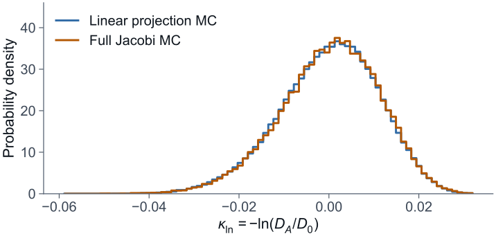
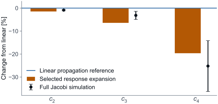
Histogram barely moves; fourth cumulant drops by 25%
linear projection vs full Jacobi, same driver change from the linear reference: \(c_2\) −1%, \(c_3\) −3%, \(c_4\) −25%
[Let the overlap land first, then advance to the cumulants.] First experiment: same driver, two propagations. The blue histogram is the exact linear law; the orange is the full Jacobi integration. They lie almost on top of each other. If you only looked at this picture you would conclude that nonlinear propagation does not matter at this amplitude. [Advance.] Now look at it cumulant by cumulant. The variance moves by one per cent. The third cumulant by three. The fourth cumulant drops by a quarter, with a sizeable error bar from fifty thousand paths. The orange bars are the diagrammatic prediction with one quadratic insertion: minus one, minus six and a half, minus twenty per cent, the same ordering and the same sign. So the propagation acts on the distribution exactly where the histogram hides it: in the tails, order by order up the hierarchy. That is the same mixing we saw in the two-point function, now read out one point at a time. c2 goes from 1.2256 to 1.2148 × 10⁻⁴ and c3 from 5.05 to 4.89 × 10⁻⁷; c4 changes by −25 ± 11 per cent against −20 per cent from the expansion with one quadratic insertion at orders 1 to 4. The banks are independent, and the linear cumulants match the analytic window to 1.5 standard errors.
Backup · Part 2 · Faraday screen cumulants
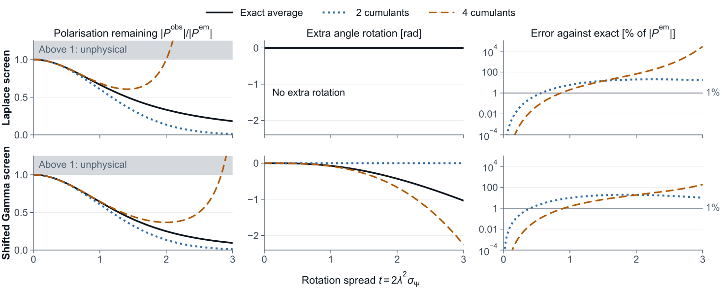
Two cumulants give one Gaussian answer for every screen; four can overshoot
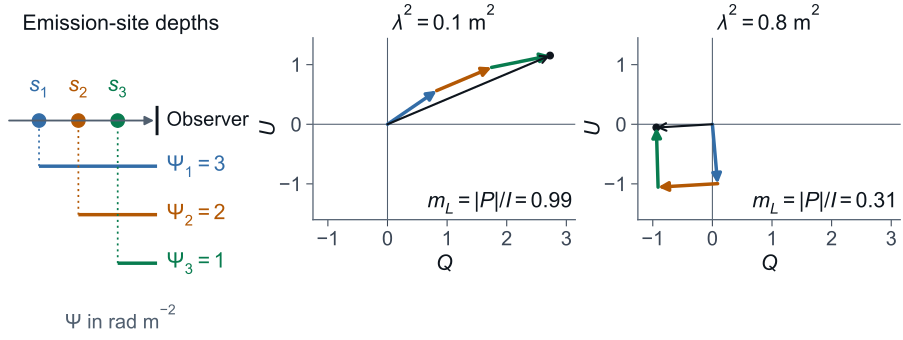
When the Faraday screen is independent of the emission its phase average factors out, and the logarithm of that factor is a cumulant series in the squared wavelength. Two cumulants give the Gaussian depolarisation for every screen with the same mean and variance, so the Laplace and skewed Gamma screens are indistinguishable at that order. Four cumulants resolve part of the difference at small rotation spread and then overshoot to amplitudes above unity. A finite cumulant list is not a probability law; that is the same lesson as in the lensing PDF. The series is log C_scr = iτΨ̄ − τ²σ_Ψ²/2 − iτ³κ₃/3! + τ⁴κ₄/4! + R₅, with τ = 2λ².
Backup · Part 2 · Correlations
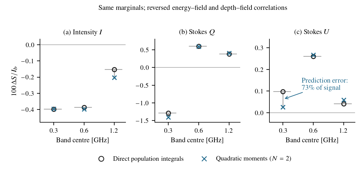
Same marginals, reversed correlations, different spectrum
Reversing the energy–field and depth–field pairings while keeping every one-dimensional marginal fixed changes \(I,Q,U\) by 0.2–1.5%. A model built from separate distributions would miss the change; the quadratic moments predict it, with a 73% error on the smallest \(U\) change at 0.3 GHz.
The joint moments retain correlations, and this is why. Two populations share the separate distributions of energy, field strength and depth but have opposite pairings. Their spectra differ by up to one and a half per cent, and a model that only used the marginals would miss the difference entirely. The quadratic moment prediction captures most of it, with the largest relative error on the smallest change, seventy-three per cent of a tenth-of-a-per-cent effect in U at three hundred megahertz. The populations are continuum distributions with 20 per cent half-widths, and the prediction error is measured relative to the size of the change.
Backup · Part 2 · What varies the spectrum
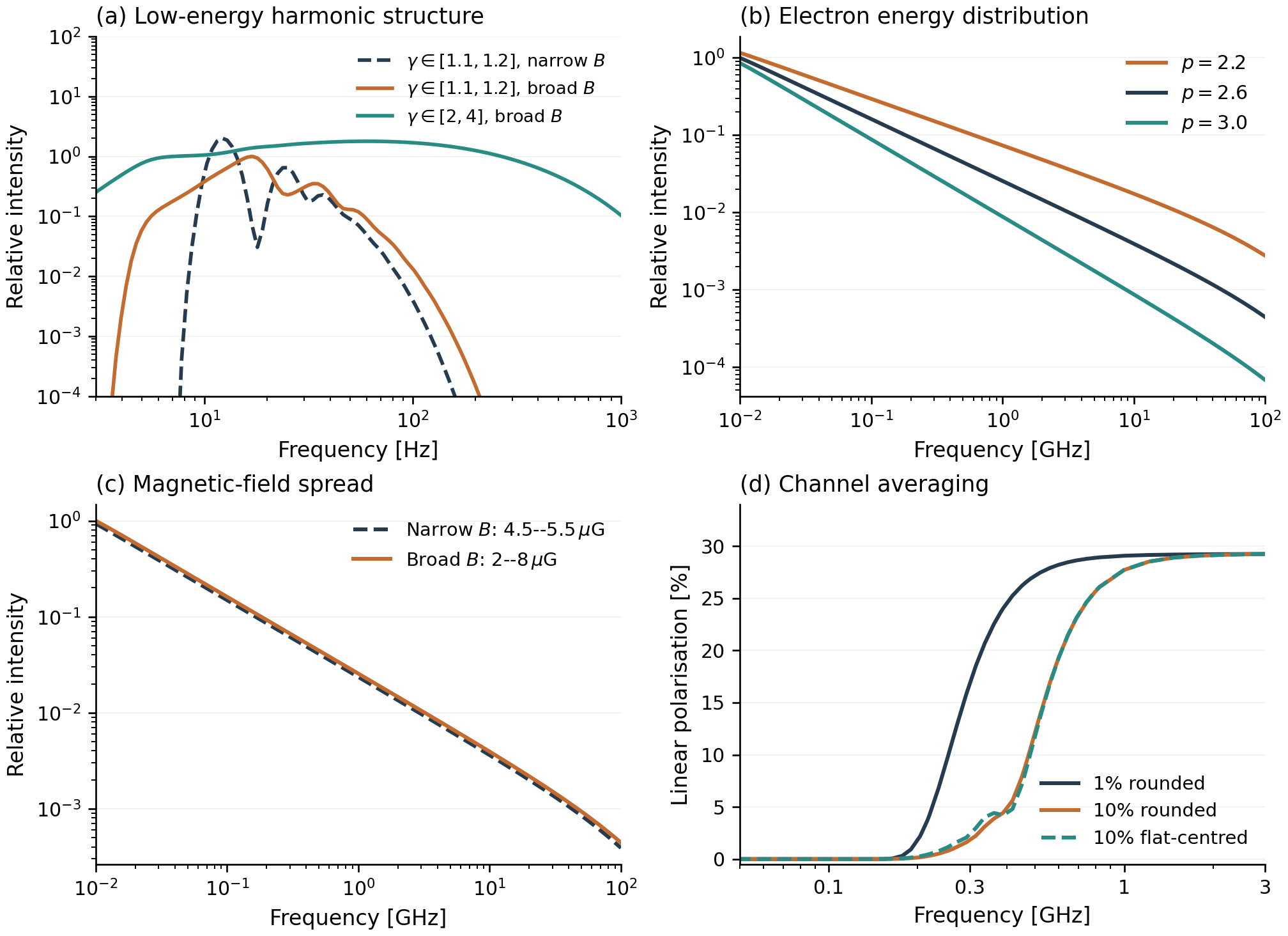
Energy index, field spread and channel width act on different parts of the spectrum
Four forward calculations. Low-energy electrons show harmonic structure that smooths out as the energy or field range broadens. The electron energy index sets the power-law slope over the gigahertz band. Doubling the field spread barely moves the intensity at fixed marginal. And the channel width decides where linear polarisation is depolarised by rotation across the band. These are the responses the moments weight.
Backup · Part 2 · Assumptions
What the emission model assumes, and where each limit is assessed
Emission helical orbit in a field uniform over the orbit; no radiation reaction; powers add incoherently; a supplied line-shape change is bounded only at fixed integrated power Propagation steady emission on one straight ray; cold-plasma Faraday rotation \(\lambda^2\Psi\); absorption, scattering, refraction and conversion omitted (scalar absorption bounded if an optical depth is supplied) Channels smooth response on a declared finite band; shifting lines and rotation integrated across the channel before expansion Population correlated energy, field and depth allowed; all moments from one nonnegative population; fitted values need the same consistency check Finite expansion finite Legendre and Taylor orders about fixed references; conditional remainder bounds; population outside the declared ranges needs a separate estimate
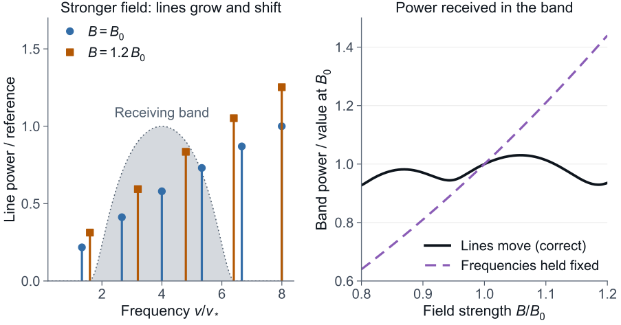
This is the manuscript's assumption table. Each row says what the calculation assumes and where its limit is assessed. The one to remember from the main talk is the channel row: a smooth channel response does not make the channel power analytic in the parameters, because a line can sit outside the channel for all parameters near the reference and enter elsewhere in the population range. Angular averaging helps; it does not guarantee convergence. Finite beams enter as a Mueller response inside the frequency integral and are not evaluated by the fixed-ray examples. A fixed-angle Taylor series in B misses entering lines: the limiting discrepancy is 12.1 per cent over B/B0 from 0.9 to 1.1 and 28.4 per cent from 0.8 to 1.2.
Backup · Part 3 · Validate the field statistics
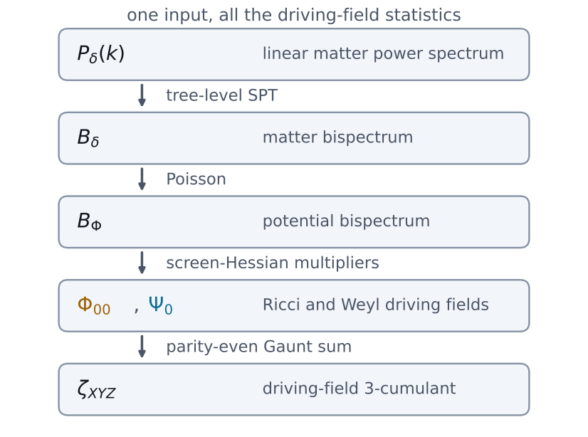
Known cumulants make the non-Gaussian test quantitative
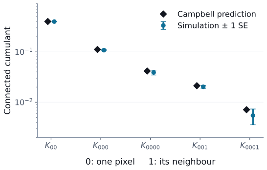
\[K_{i_1\cdots i_r}=\lambda a^r\sum_j B_{i_1j}\cdots B_{i_rj}\]
For \(r\ge3\), Campbell's theorem: connected sky cumulants of the Poisson component; the Gaussian part contributes only at \(r=2\). \({K_3\propto\lambda^{-1/2}}\), \({K_4\propto\lambda^{-1}}\). Beam coupling predicts one-pixel and neighbouring-pixel statistics.
Before using the Poisson-Gaussian density for inference, its cumulants are checked against simulation. Campbell's theorem gives the connected cumulants in closed form, with the third scaling as one over root lambda and the fourth as one over lambda. The one-pixel and neighbouring-pixel cumulants agree with a hundred thousand realisations within one and a half standard errors. The simulation has 98,304 realisations, and all five checks fall within 1.42 standard errors.
Backup · Part 3 · Gaussian reference, non-Gaussian target
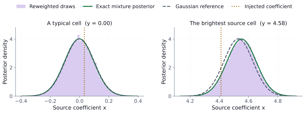
Same Gaussian draws, a non-Gaussian posterior
Each draw keeps its position; its weight \(w_m(\lambda)=p_\lambda(x^{(m)},d)/p_0(x^{(m)},d)\) changes its contribution. Factorised weighting is valid here because the observation \(d=B(x+\epsilon)\) with invertible \(B\) and source-coordinate white noise makes both reference and target factorise cell by cell; a general beam-correlated noise does not.
The reweighted draws sit on the exact mixture posterior, both in a typical cell and in the brightest source cell where the Gaussian reference is visibly off. The factorisation that makes the whole-map weight collapse harmless is a property of this controlled model: an invertible beam and noise that is white in source coordinates, before the beam, make both the reference and the target factorise cell by cell. Main slide 38 uses the same construction. With noise that is white after the beam, and therefore correlated in source coordinates, that would not hold, and the whole-map weights would have to be used. The two-cell posteriors come from the saved banks. The whole-map effective sample size is 6 of 2,048.
Backup · Part 3 · The computational engine
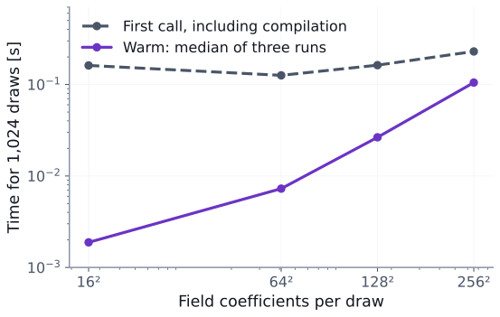
A tractable reference makes a large sample bank cheap
0.105 s
1,024 Gaussian field draws of 65,536 coefficients; warm JAX CPU, float32
\[p_0(x\mid y)=\mathcal N\!\Big(\frac{y}{1.01},\frac{0.01}{1.01}I\Big)\]
closed-form diagonal GCR conditional in source coordinates, \(y=B^{-1}d\)
How cheap can the reference bank be? In source coordinates the Gaussian conditional is diagonal, so the draws are independent and a thousand fields of sixty-five thousand coefficients take a tenth of a second warm. The dashed line includes compilation. This timing covers drawing only; weights and beam transforms are separate, and it is not a comparison with any sampler.
Backup · Part 3 · Bayesmith
Is an exact block always better than NUTS?
Sampler Budget max |pull| factor sweep 600 + 900 8.46 factor sweep 2400 + 3600 4.10 pure NUTS 600 + 900 1.05 pure NUTS 2400 + 3600 0.97
Worst replication of a seven-parameter hierarchical model; pull = (posterior mean − truth) / posterior SD. Each conditional draw in the sweep is exact, but alternation between strongly coupled blocks mixes slowly; NUTS with an adapted mass matrix moves along the coupling. The documented use of the sweep is an exact block too large for gradient sampling, such as a sky map or per-channel gains.
No. Each conditional draw in a Gibbs sweep is exact, but alternating between strongly coupled blocks mixes slowly, and in this seven-parameter model the sweep is biased by several posterior sigmas at the same budget where NUTS is fine. The documented use of the exact block is the case where the block is too large to gradient-sample, a sky map or per-channel gains. The plan Bayesmith prints is a choice you can audit, not a guarantee of efficiency. The composed-process run corrects its proposal with Metropolis–Hastings against the full model.
Backup · Part 3 · RHINO calibration
A gradient gives the response; identifiability is a rank test
\[\mathrm{rank}=\min(n_{\rm src},k)\times n_{\rm freq}\]
One equation per switch position per channel; \(k\) free temperature families. Three sources make a three-family fit square and leave a four-family fit short by \(n_{\rm freq}\). Calibration on simulated data with 24 free noise-wave temperatures: Wiener mean by conjugate gradients, RMS errors 0.13 / 0.11 / 0.11 K on spreads of 40 / 60 / 8 K; condition number 40 with three sources, \(4\times10^6\) with one, and the solver refuses. Adding two foreground parameters to the four-family twin gives nullity 2 of 34 and the plan refuses to run; three more loads and seven switch positions restore nullity 0.
A gradient is not identifiability. Each switch position gives one equation per channel, so the rank is the smaller of the number of sources and the number of free temperature families, times the channels. The simulated calibration recovers twenty-four noise-wave temperatures with RMS errors of a tenth of a kelvin, and the solver refuses when the design is degenerate. Adding foreground parameters to the same twin makes it degenerate; more loads and switch positions repair it. Twelve of the twenty-nine operator classes carry physics; the rest are placeholders with tested interfaces, and nothing has been validated on real data yet. The calibration is simulated, with fixed sky and beam.
Backup · Part 3 · rheplicant-agent Workbench
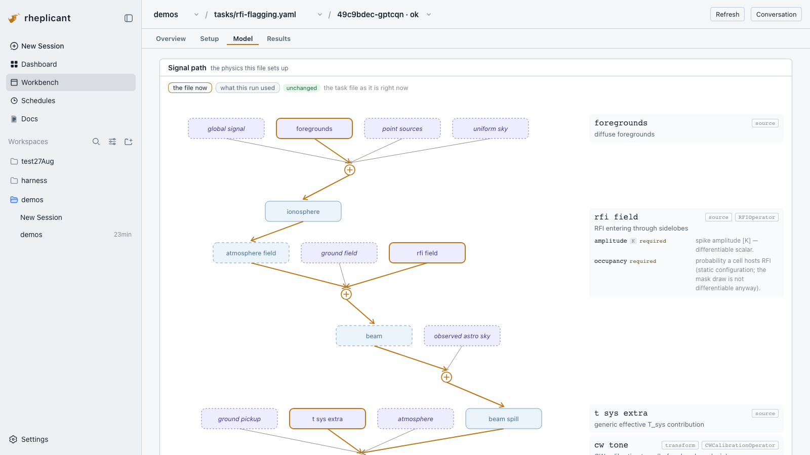
The task file read as a signal path
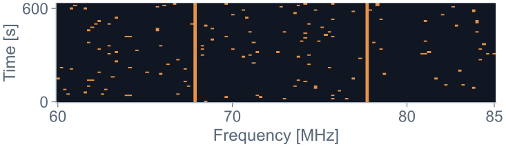
The Workbench shows a task file as the physics it sets up. The stages this run used are highlighted along the signal path: diffuse foregrounds, the RFI field entering through the sidelobes, an extra system temperature, a CW calibration tone, noise, and the flagging operator at the end. The right-hand column lists each operator's parameters and says which are differentiable; the RFI occupancy is not, because the mask draw is discrete, and the file says so. The Setup and Results tabs hold the same run's configuration and products.
Backup · Part 3 · rheplicant-agent Flags panel
Before and after flagging, on one colour scale
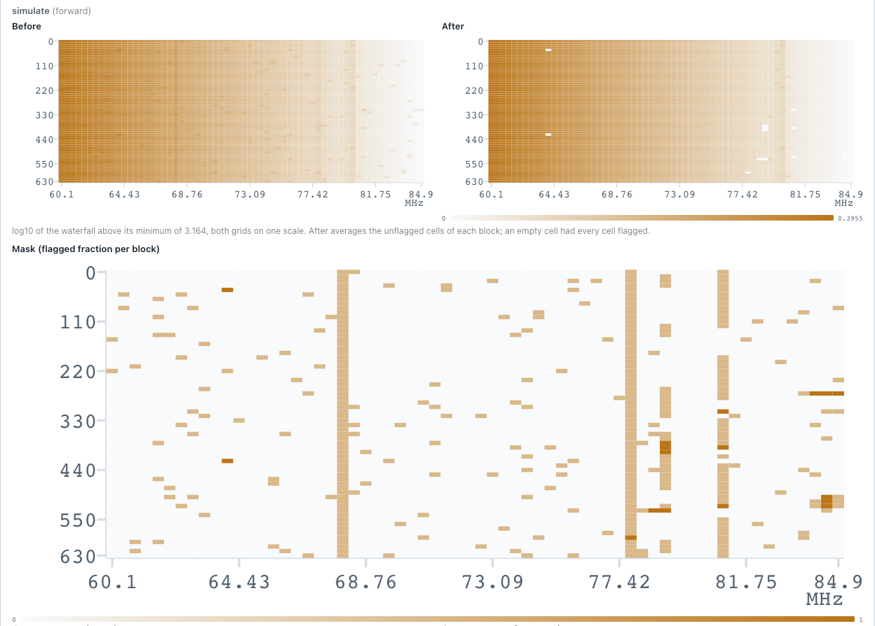
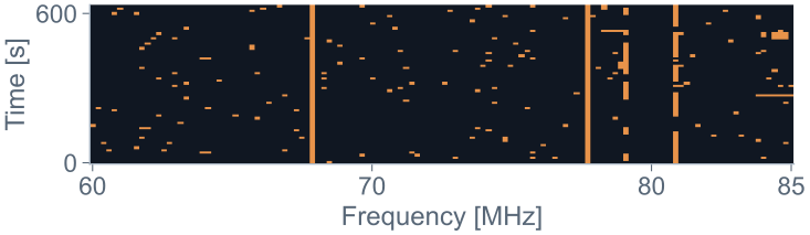
The Flags panel: the simulated waterfall before and after the fourth round on one colour scale, and the mask underneath. The persistent RFI channels are the vertical lines; the scattered blocks are single bursts. The statistics the checks are computed from sit below the plots in the same panel. The run is execution 49c9bdec-79gqfg after round 4. Colour is log10 of the waterfall above its minimum, and 'after' averages the unflagged cells of each block. The run flags 4.57 per cent of the 64 × 128 blocks, none in the 8 protected channels; the residual excess kurtosis is 0.52, and a re-fit reproduces the mask.
Backup · Part 3 · rheplicant-agent session
The chat that drove the four rounds
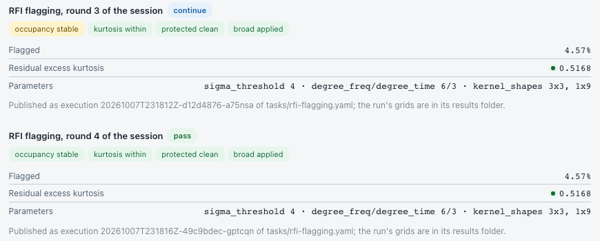
This is the session view of the same four rounds, from the earlier capture. Each tool call comes back as a card: the verdict, the four check badges, the flagged fraction, the residual's excess kurtosis, the parameters used, and the execution it published. The guidance rules tell a model to start loose, tighten, then add the broad kernels, and to stop at pass; here the tool was run with exactly that sequence, without a live model; the checks themselves are computed by the tool. Sigma goes 12, then 4, then 4 with the 3×3 and 1×9 kernels, the sequence the six guidance rules prescribe. The capture replays recorded tool executions without a live language model. The capture predates the timeline commit, so its execution ids differ from the Results tab's run.
Historical backup · Part 3 · Demo C identifiability
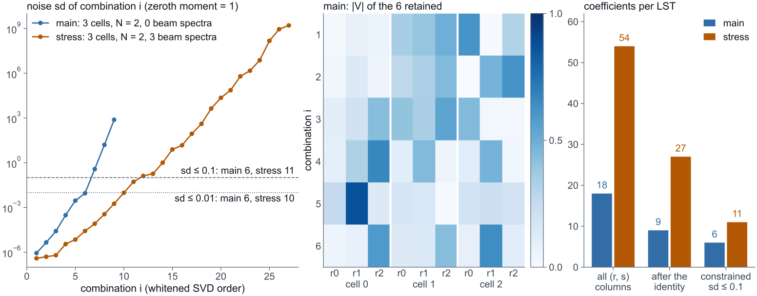
Six constrained combinations per LST, out of eighteen columns
[Historical: Demo C, the per-LST spectral fit of an earlier version of this talk.] Which coefficient combinations does one sidereal time's spectrum constrain? The field-derivative columns go first, by the exact scaling identity of part two: eighteen columns become nine. Then a noise-whitened singular value decomposition: six combinations have a noise standard deviation below a tenth of the zeroth moment, and sharing the coefficients across the ninety-six LSTs adds one more. The remaining three are unconstrained by this band at this noise, and the posterior integrates over them. The zeroth moment is normalised to 1 and the noise is 10 mK. The identity C01 = C00 + C10/2 holds to 10⁻¹⁶. In the stress basis the counts are 54, 27 and 11.
Historical backup · Part 3 · Demo C in the stress band
Where no per-LST spectral basis passes
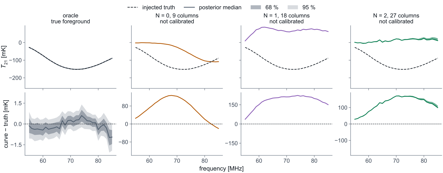
[Historical: Demo C.] The stress band is where Demo C fails. With one-megahertz channels and the wet-horn beam, the chromaticity defeats every per-LST spectral basis: none of the eighty-two candidates passes the fit check, and the fallback basis spends twenty-seven columns on thirty-one channels and still misses the trough. The ad hoc moment basis fails the same way. Only the sky-map strategy, which models the chromaticity through the beam rather than through the spectrum, stays calibrated there. The stress scenario has 1 MHz channels over 55 to 85 MHz with the HornWet beam. The fallback basis (K = 3, N = 2, 3 beam spectra) has σ(amp) 2.17, against 3.01 for Demo A and 1.71 for Demo B.
Backup · Part 3 · A controlled non-Gaussian sky
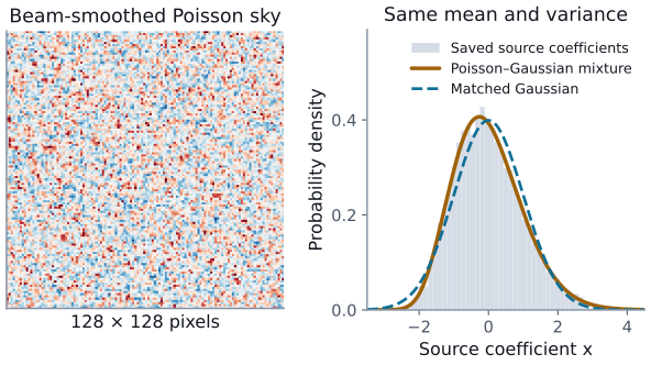
Same power spectrum, different source populations
\[x_j=a(N_j-\lambda)+g_j,\quad N_j\sim{\rm Pois}(\lambda)\]
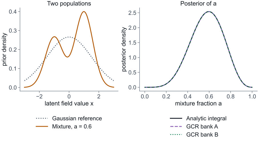
With \(a=\sqrt{0.8/\lambda}\), for every candidate \(\lambda\): \(\mathbb E[s]=0\), \(\mathrm{Cov}(s)=BB^{\mathsf T}\). Rare bright sources or many faint ones: the covariance cannot tell. The higher cumulants can, and Campbell's theorem gives them in closed form.
Part one's shot-noise drive as a sky to be inferred: recover \(\lambda\) from a 16,384‑coefficient map.
The same construction as part one's shot-noise drive: Poisson events plus a Gaussian background, with the amplitude chosen so that the mean and covariance are the same for every event rate. Here it is a sky on a hundred-and-twenty-eight-squared grid seen through a beam, and the rate is the thing to infer. The covariance cannot see it; the third and fourth cumulants can, and Campbell's theorem gives them exactly. The diffuse Gaussian has variance 0.2 and the injected rate is λ = 2. Analytic cumulants agree with 98,304 realisations within 1.42 standard errors.
Backup · Part 3 · Marginalise the field, infer its population
Recover the source rate, and check the weights
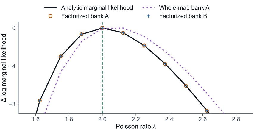
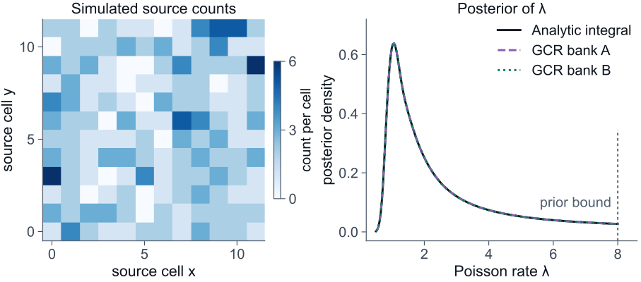
16,384 latent coefficients · rate MAP 2.0014 · analytic 2.0015 · injected \(\lambda=2\)
\[w_m(\lambda)=\frac{p_\lambda(x^{(m)},d)}{p_0(x^{(m)},d)}\]\[\frac{Z_\lambda}{Z_0}\simeq\frac1M\sum_m w_m(\lambda)\]
Draw the Gaussian reference bank once ; every candidate \(\lambda\) only changes the weights. 1,024 draws of 65,536 coefficients cost 0.105 s.
Whole-map weights collapse : ESS 6.2 of 2,048. The exact source-coordinate independence of this model factorises the estimator; minimum local ESS 1,614 of 2,048, and two independent banks agree with the analytic curve.
A cheap Gaussian reference: draw a bank of fields from the Gaussian conditional once, then every candidate rate only changes the importance weights. The recovered rate is two point zero zero one four against an injected two. With whole-map weights the effective sample size collapses to six draws out of two thousand; the controlled model's exact source-coordinate independence factorises the estimator cell by cell, and the local effective sample size is sixteen hundred. Efficient inference needs cheap draws and usable weights, and the second is a property of the model that has to be established. The prior on λ is uniform. [Relation to main slide 38.] Slide 38 is the same construction on a 12 × 12 grid with whole-field weights; this earlier, larger run on a 128 × 128 grid needs the factorised estimator.
Part 1 · Path-integral weak lensing · How solid
The amplitude still rises with the cutoff; the observable is fixed
Held fixed in the number
Source single plane, nominal \(z_s=5\) Path Born; scalar-only, \(\Phi=\Psi\) Driver linear \(P\), tree-level SPT bispectrum Cutoff vertex \(\ell_{\max}=15360\) Readout raw \(\langle\kappa_1\kappa_2\rangle\) moment, linearized map
What moves it
UV sensitivity. A collapsed configuration is a coincident-point moment. On the post-fix cutoff ladder the last doubling of \(\ell_{\max}\) still adds 17% at 0.5′ and about 9–11% in the band at tree level, and 103% at 0.5′ with BiHalofit. No cutoff-independent nonlinear amplitude is quoted: slide 21's 5–10% is the \(\ell_{\max}=15360\) value, still rising.
Spin signature. Linear scalar lensing is pure E in every realisation, so \(\Delta C_\ell^{BB,\,FK}=2\,\mathrm{Re}\langle B^{(1)}B^{(2)*}\rangle=0\). FK changes E only; the first allowed B-mode is Gaussian FF at field order 4.
Readout. Jacobi \(\kappa_A\), reduced shear and the source sample are external insertions still to be folded: the other stations of the complete view.
[Backup; what the number holds fixed and what would move it.] Left: what the number holds fixed; it is on the slide, I will not read it. Right: what would move it. First, ultraviolet sensitivity. A collapsed configuration is a coincident-point moment, so it is UV-sensitive by construction. On the cutoff ladder of 5 October, the last doubling of the cutoff still adds 17 per cent at half an arcminute and about 9 to 11 per cent in the band at tree level, so the tree-level amplitude still rises with the cutoff. At ell max 15360 that ladder reads 1.34 to 1.40 per cent in the band at tree level, below the 1.43 to 1.50 per cent of slide 20. With the BiHalofit bispectrum the last doubling adds 103 per cent at half an arcminute, so the sum has not converged by ell max 15360, and I quote no cutoff-independent nonlinear amplitude; the 5 to 10 per cent of slide 21 is the value at ell max 15360, still rising. [If asked: the ladder is a saved product of 5 October, accepted for finite amplitudes and sampled signs only, not as a scientific result. It sits at the true redshift-5 plane, with the 3 October spin-2-corrected vertex tables and sft-wick 0.6.1. Slide 20 is the 12 September fold at the nominal plane, with sft-wick commit a4befdc, which merged the nonlocal-coupling leg-order fix on 11 September; its vertex table was rebuilt on 6 September and has a recorded leg-symmetry check. No post-fix redshift sweep exists. The direct Monte Carlo check of the fold in the backup dates from 28 August, before the leg-order fix.] [Advance.] Second, the spin signature. FK changes E only: its linear leg is pure E, so its B-mode contribution vanishes. The first allowed B-mode is the Gaussian FF term, at fourth order in the source field. [Advance.] Third, the readout. The Jacobi convergence, reduced shear and the source sample are external insertions that have not been folded yet. The complete-view backup shows where they enter.
Part 1 · Path-integral weak lensing · Beyond two-point statistics
The one-point law reads what the covariance cannot
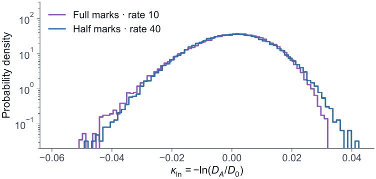
same driver covariance, half the marks × four times the rate: skewness 0.37 → 0.18 same driver, linear vs full Jacobi propagation:
Same power spectrum, different laws: the skewness halves. Nonlinear propagation moves the fourth cumulant by a quarter while the variance moves 1%.
[One slide; it is the same lesson one point at a time.] The two-point function is one readout of this chain. Here is the other, in a model where every link is specified exactly: discrete curvature events along the ray with a known positive law, propagated through the full Jacobi equation, read out as the log of the angular-diameter distance. The events are compound-Poisson with exponential memory; the full Jacobi runs use 50 thousand paths, the exact linear law 200 thousand. The law is not calibrated to a cosmology. Left: halve every kick and quadruple the rate. The driver covariance is unchanged, so a two-point analysis sees nothing, and the two histograms look almost the same; but the skewness of the output halves and the kurtosis drops by a factor of three. That is the shot-noise picture from the toy, now after full optical propagation. [Advance.] Right: keep the driver and change only the propagation from linear to full Jacobi. The variance changes by one per cent, but the fourth cumulant drops by a quarter: white points are the full simulation, orange bars the one-insertion diagrammatic prediction. Propagation acts where a histogram hides it: in the tails, order by order up the hierarchy. The same machinery organises both readouts.
Part 1 · Path-integral weak lensing · A complete view of the corrections
Corrections enter at every station along the ray
Driving fields · large-scale structure nonlinear growth · connected cumulants κ⁽²⁾, κ⁽³⁾, κ⁽⁴⁾ … · unresolved small-scale structure observer source galaxy Ray path beyond-Born: curvature on the bent ray radial and time shifts Screen & frame transported basis, tilt frame rotation ≠ image rotation Beam propagation lens–lens coupling, nonlinear Sachs response: FF and FK Image & observable reduced shear g = γ/(1−κ), magnification finite-source flux, size and shape Source endpoint fixed zobs ≠ fixed affine distance source and observer frame terms Catalogue sample source clustering, magnification bias weights and normalisation Mixed terms: path × propagation · bispectrum × response · reduced shear × selection · endpoint × sampling · intrinsic shapes × lensing[Build the picture in three steps; do not read every label.] [The map follows the Unify-WL design (Oct 2026).] We now have machinery that computes contributions. Step back: what does a complete higher-order prediction contain? The input is the driving statistics along the top: nonlinear growth, the connected cumulants, unresolved small-scale structure. [Advance.] Along the ray, three stations. The ray path: curvature evaluated on the bent ray, the beyond-Born family. The screen: the basis is transported and rotates, and frame rotation is not image rotation. And the beam: successive tidal couplings and the nonlinear Sachs response, where lens-lens coupling and our FF and FK channels live. [Advance.] Then the readout. At the observer, the image: reduced shear, magnification, finite-source response. At the source, the endpoint: fixed redshift is not fixed affine distance. And the catalogue: clustering, magnification bias, weights. [Advance.] Finally the mixed terms: path with propagation, the bispectrum with the nonlinear response, reduced shear with selection, intrinsic alignments with lensing. Familiar names such as post-Born straddle these boxes, so this is an origin map, not a list of additive corrections. The rest of this part opens one corner of it: the driver statistics through the nonlinear beam propagation, read out first as a two-point function and then as a one-point distribution. [If asked: screen rotation, optical twist and image rotation are three distinct effects.]
Backup · Part 2 · The accuracy we need
Judge the model error in the space of the science parameter
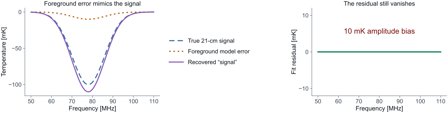
10 mK → 0
signal-shaped foreground error: 10 mK amplitude bias, zero residual
A finite-moment error is small or large only relative to the signal it mimics. Propagate it through the observing response and the estimator, not the raw residual.
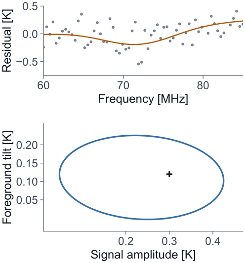
[Backup; Q&A crib for the question of what accuracy a foreground expansion needs.] Why does the accuracy of a foreground expansion matter in this particular way? Because the quantity we extract is not the spectrum but a signal amplitude fitted through a foreground model. A ten-millikelvin foreground error with the shape of the signal shifts the inferred amplitude by ten millikelvin, and the fit residual is exactly zero. [Advance.] So a moment truncation error must be judged after propagation through the observing response and the estimator, in the space of the science parameter, not by how small the residual looks. To do that for a real experiment, the sky model has to be carried through the instrument and into an inference. [If asked.] The figure is an exact template-degeneracy illustration; it shows no measured synchrotron mismatch. Population-model benchmarks against a 78 MHz absorption template are in the manuscript's extended discussion.
Historical backup · Demo C (per-LST spectral fit) compiled by bayesmith
Demo C's plan: a tolerance the arithmetic cannot reach
block 0  {fg_coeff}   GCR exact   structurally certified;
         numerical check 3 scales x 3 at-points (max 0.00e+00)
         kappa=1e+14 -> tol=1e-17 ... tol UNATTAINABLE at this
         dtype: the condition bound times the machine epsilon
         is 0.0222, already past the 0.001 target ... Run inside
         `with jax.enable_x64(True):` ... or strengthen the prior
block 1  {u}          NUTS
         outside the exact block ['fg_coeff']: sampled by NUTS,
         and the exact block is solved CONDITIONAL on them,
         once per sweep
execution: HMCGibbs(inner=NUTS, gibbs_sites=['fg_coeff'])
The graph: \(c\), 96 LST × 9 foreground coefficients, Gaussian prior; \(u\), 7 box-mapped 21-cm parameters through an emulator; waterfall \(\sim\mathcal N(c\,\Phi^{\mathsf T}+T_{21}(u),\,10\,\mathrm{mK})\). Nothing was declared : the affine block was found in the traced program, then checked numerically.
Gaussian conditional solve, draw (GCR) or integrate out analytically; the plan also says when the arithmetic cannot deliver the tolerance
Useful local structure log-space, iterative GLS or Gauss–Newton proposal, corrected to the full target by Metropolis–Hastings
General dependence NUTS; a gradient route returns a convergence certificate (Newton decrement) or refuses with a reason
[Historical backup; the plan bayesmith printed for Demo C, the per-LST spectral fit of an earlier version of this talk, no longer in the main deck.] This is the plan it prints: per-LST foreground coefficients on a fixed basis, and seven twenty-one-centimetre parameters through an emulator. Block zero, the coefficients: an exact Gaussian draw, certified from the program and checked numerically. Then a warning: with the flat-like prior I gave the coefficients, the condition number is ten to the fourteen, so even in double precision the inner solve cannot reach its tolerance; the plan says so and suggests a stronger prior. Block one, the signal parameters: NUTS, with the exact block solved again once per sweep. Demo C's posteriors took the shortcut the first line allows: the twin integrated the Gaussian block out exactly, then ran SMC. Nothing about the coefficients was declared; the affine structure was found in the traced program and verified. [Advance.] The routes are ordered by how much is exact: a Gaussian conditional is solved, drawn or integrated out; a local Gaussian proposal is corrected by Metropolis-Hastings; [advance] everything else goes to a gradient sampler, and a gradient fit returns a convergence certificate or refuses with a reason. When an early compile got this wrong, the refusal said why, and the fix was one line. [If asked.] The printout is abridged. The first compile put both latents in one NUTS block because the prover refused four primitives on the 21-cm path (erf, erfc, custom_jvp, scan) that the block never reaches; the gate is fixed on main. A 10 to the 5 kelvin prior on the coefficients makes the inner tolerance unattainable in float64; a 10 to the 3 kelvin prior makes it attainable.
Backup · Part 2 · The sky models we have
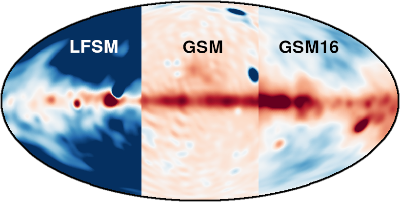
Sky models disagree at the 10 % level
LFSM · GSM · GSM16, one sky, three models > 10 %
disagreement between the models, as quoted in the RHINO overview
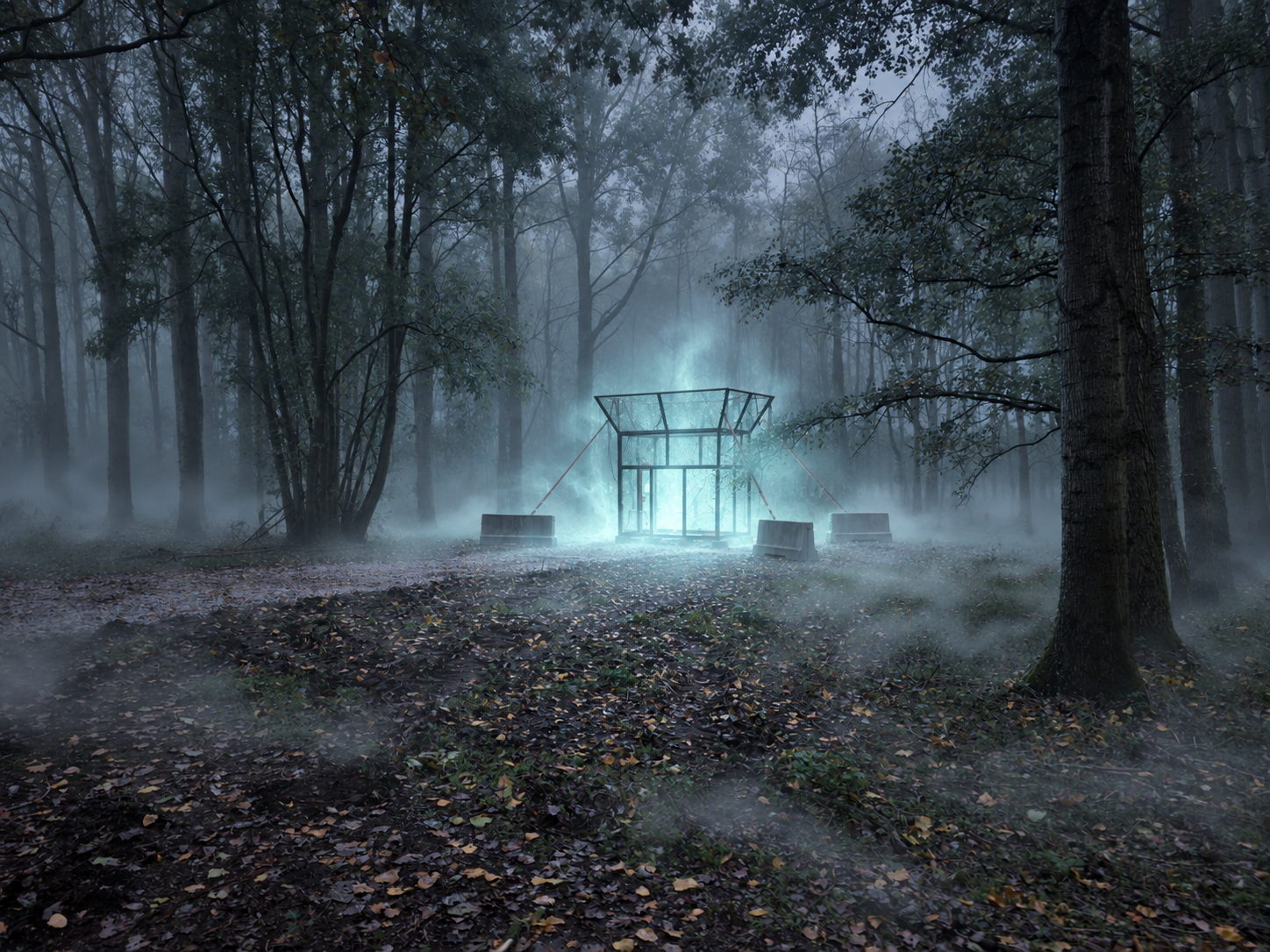
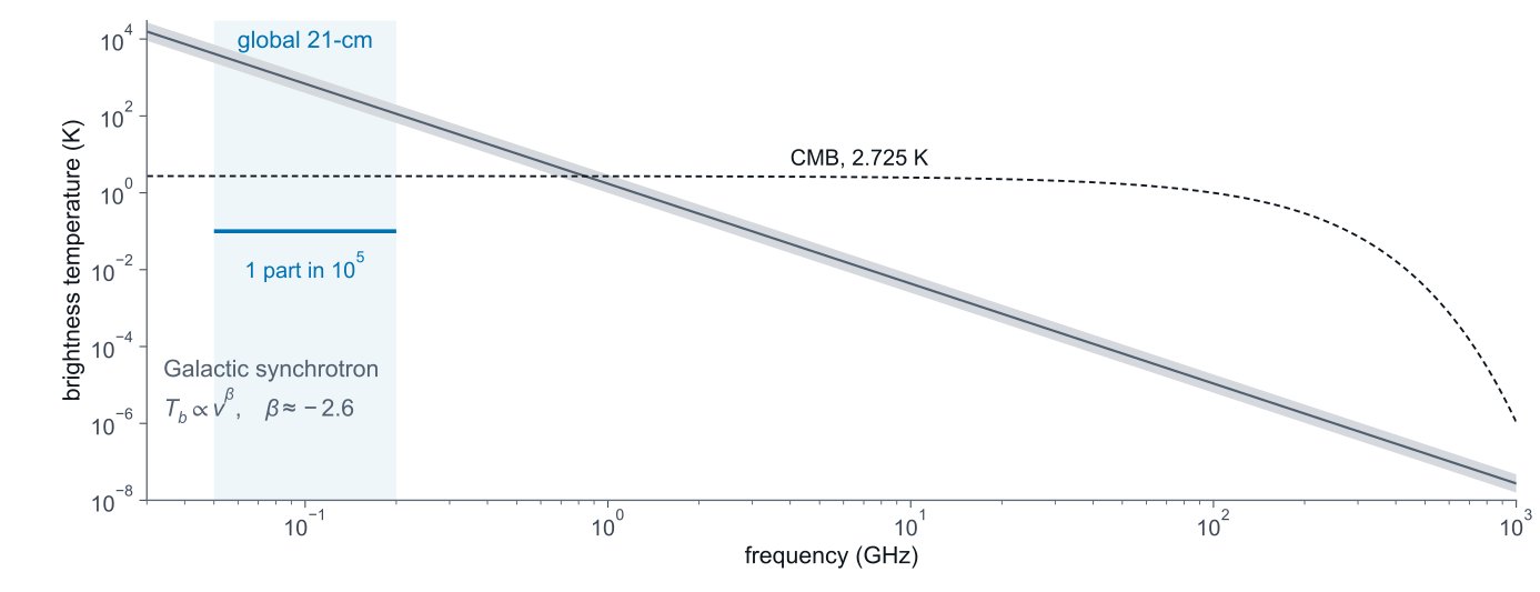
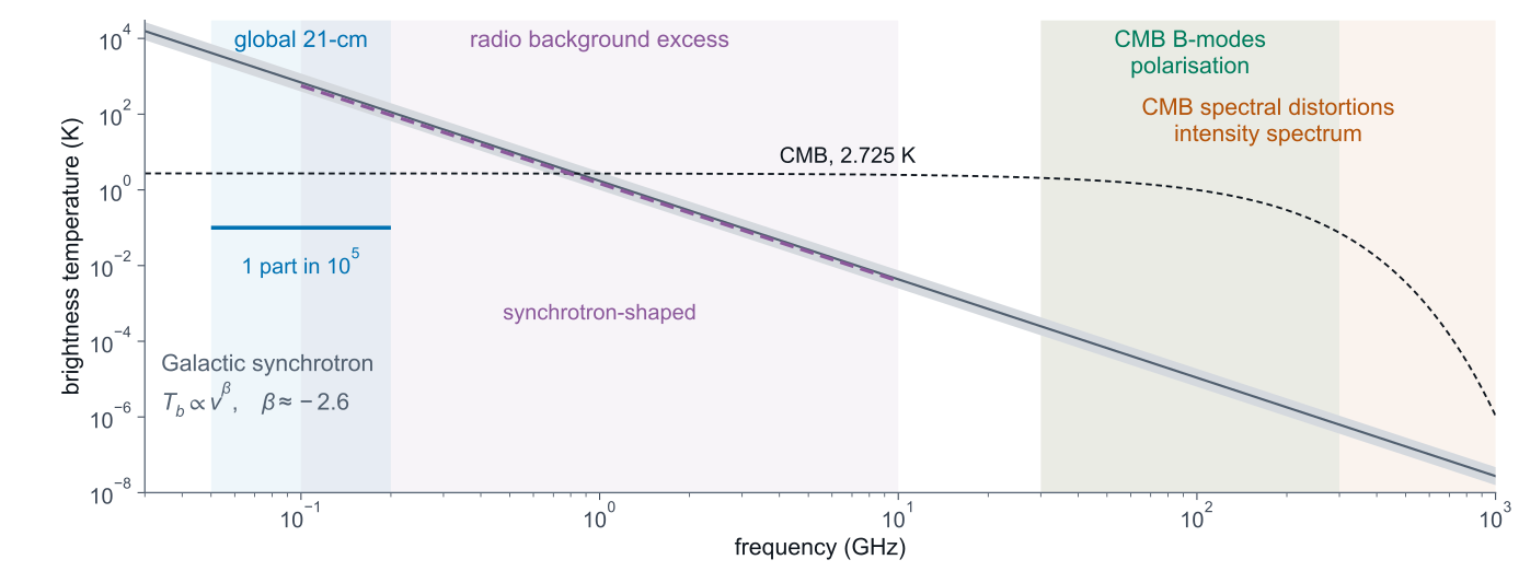
A global 21-cm model has to be good to about one part in a hundred thousand for the model error to stay below the signal.
[Backup to slide 24.] The three sky models of the same sky, LFSM, GSM and GSM16, disagree with each other by more than ten per cent, while the model error that a 100 mK signal under thousands of kelvin tolerates is one part in a hundred thousand. The map is from Phil Bull's RHINO overview, slide 23, credited there to Irfan et al. 2023. That slide states neither the plotted quantity nor the frequency, and the image has no colour bar; the ten per cent is the overview's text.
Backup · Part 3 · bayesmith routes
Five routes a block can take
method printed as meaning
gcr GCR exact exact conditional Gaussian draw; the noise does not move with the block gcr+snis GCR + SNIS whole graph exact, noise moves with it: GLS fixed point, corrected by self-normalised importance sampling gcr+mh GCR + iterative GLS + MH exact block beside a sampled remainder with moving noise: the exact draw is an MH independence proposal log-gcr log-gcr the exact draw on a log-transformed block whose prediction is exponential in an affine function nuts NUTS NumPyro's No-U-Turn sampler
One Gaussian conditional supports three operations: solve, draw, integrate out. Which structure takes which route: linear-Gaussian with an eligible covariance, a supported log-linear form, conditionally Gaussian affine groups inside a chain, an eliminable exact block with a sampled residual, a general differentiable model.
[Backup; the method table from the documentation.] A plan partitions the latents into blocks and gives each one of five methods. The exact routes need an affine prediction, a Gaussian prior and a noise that does not depend on the block, established twice: a structural certificate over the traced computation and a numerical probe at three scales and three points. A mixed plan runs NUTS on the sampled block and draws the exact block once per sweep. The five typed questions a graph can be asked are Posterior, Evidence, Predictive, PointEstimate and Simulation; each returns a Result of the same name or a Refusal. Related: the existing page on whether an exact block is always better than NUTS.
Backup · Part 3 · bayesmith Example 03
Example 03: chains and provenance
Hierarchical-model recovery · recorded all-NUTS run
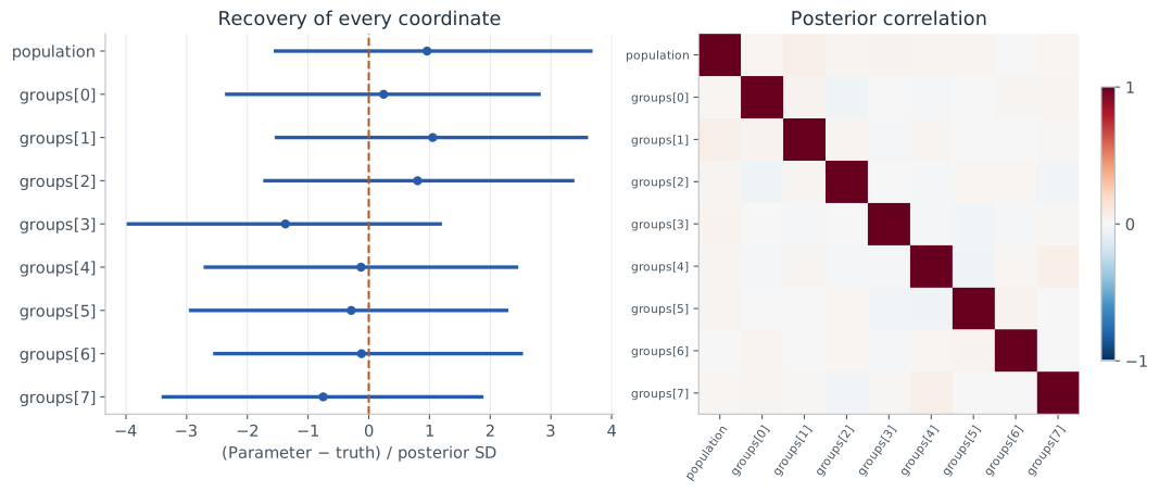
chains × draws 2 × 2,000 after 1,000 warmup, seed 0 divergences 0 population R-hat 1.000004 population ESS 8,817 population mean 1.008 ± 0.217, truth 0.8 run record plan, fingerprints, seed, dtype, devices, backend, budget, termination, approximation class refusal failed premise, grounds, scope, remedies, optional fallback
[Backup; bayesmith's Example 03, a hierarchical model with group means, from the package documentation; not one of the main-deck examples.] The figures are a snapshot of an earlier all-NUTS run on 0.9.0; 0.10 compiles the same declaration to a mixed plan, not shown in this talk, with the group means solved exactly inside NUTS. The single-case recovery and these chain diagnostics do not establish simulation-based calibration. Every result carries its run record and is reused or invalidated by fingerprint.
Backup · Part 3 · The RHINO pipeline
RHINO's open-source pipeline
rhino-daq PFB spectrometer and Arduino control driver
momentRFI RFI flagger: iterative clipping and 2-D surface fitting
rhino-cal noise-wave fitting, Kirkham+ method
rhino-monitor live satellite, weather and plane monitor
rhino-sparams lab measurements
rhino-beams beam simulations
husky Bayesian sky model, simple foreground fits
rheplicant digital twin, live simulation; inference on bayesmith
[Backup; where the twin sits in the experiment.] The RHINO overview groups the pipeline into: acquisition, RFI flagging, noise-wave calibration, monitoring, lab measurements and beam simulations on the instrument side; a simple Bayesian sky model, the Bayesian map-maker limTOD, and rheplicant, the twin whose inference runs on bayesmith. The same overview also lists hydra-global, a Gibbs sampler for noise-wave calibration; its repository under HydraRadio is a placeholder without code, so it is not on this page.
Backup · Part 3 · Spectral maps · What a log fit measures
A log fit through a beam returns brightness-weighted moments
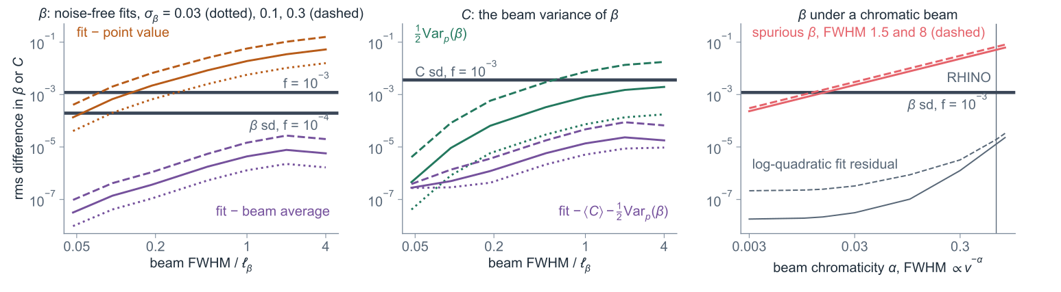
\[\ln d_p=\ln\tilde T_p-\langle\beta\rangle_pL+\big(\langle C\rangle_p+\tfrac12\mathrm{Var}_p\beta\big)L^2-\big(\tfrac16K_{3,p}(\beta)+\mathrm{Cov}_p(\beta,C)\big)L^3+O(L^4)\]
moments weighted by \(B_{pq}T_q(70\,\mathrm{MHz})\) · noise-free fits of the simulator sky through Gaussian beams · sd bands from the beam-smoothed prior Fit − moment: \(2.7\times10^{-5}\) (β) and \(8.8\times10^{-5}\) (C) rms; ½Var ≥ 0; fit residual ≤ \(8.7\times10^{-6}\); cubic term against its prediction: correlation 0.9996. A pivot at 60 MHz moves β by 0.022 rms. Chromatic beam: spurious β grows by 0.0077 rms per 0.1 in α. Smoothing every channel to the widest beam restores the moments without noise; with noise it is untested.
[Backup; what β and C mean when the beam averages over the sky.] Write the data as the log of a beam-weighted sum of power laws and expand in L about 70 MHz. The weights are the beam times the sky at 70 MHz, so every moment is brightness-weighted. The slope is the mean β; the curvature is the mean C plus half the variance of β inside the beam, which is never negative; the cubic term carries the third cumulant of β and its covariance with C. The left panel shows the fit against both readings for three amplitudes of the β field: against beam averages the difference stays below 10⁻⁴, against point values it crosses the posterior sd. From these noise-free fits the point reading of β holds, with a bias below the posterior sd, for beam widths below about 0.13 of the coherence length at f = 10⁻³ and about 0.05 at f = 10⁻⁴ (β field amplitude 0.1). The middle panel shows the half-variance term in C. The right panel shows a chromatic beam: the spurious β is linear in the chromaticity and the fit residual stays far below the noise, so the residuals do not reveal it. Changing the pivot frequency changes β by the curvature term, and the refit equals the moment at the new pivot. Smoothing every channel to the widest beam removes the chromatic term in noise-free fits; it was not tested with noise. Noise-free prediction against full run: the posterior mean of noise-free data plus the noise variance of that mean differs from the four full runs on the limits slide by up to 3.5 per cent against point values and 10.3 per cent against beam averages.
Backup · Part 3 · Spectral maps · Exactness and cost
The block is exact; converged NUTS means differ by ≤ 0.15 sd
check unknowns result
Fourier modes, 1 and 4 visits 12,288 sd ratio 0.988–1.002 dense oracle 768 mean ≤ \(4.8\times10^{-5}\) sd; sd ratio 0.990, 1.003 dense Cholesky, t eliminated 12,288 mean ≤ \(3.8\times10^{-5}\) sd; sd ratio 0.995, 0.998 NUTS, f = 0.001, 0.03, 0.0599 108 two chains: means within 0.10, 0.14, 0.15 sd; sd ratio 0.976–1.001 log step, f = 0.06, 0.07 108 refused (fractional_too_large) NUTS, uniform 432 within 0.12 sd; R-hat ≤ 1.01; 0.84–0.89 s per effective draw NUTS, scan stripes 432 not converged: R-hat up to 1.092 (β); ESS down to 13.6 (C) 128 × 128, end to end 49,152 11.9 s per draw; z rms 1.08, 1.04
beam-smoothed prior · NUTS: dense mass, 1000 + 1000 steps Certified CG runs: relative error ≤ \(5.0\times10^{-4}\). Operator records at \(f=10^{-3}\)–0.0599: \(\kappa\le6.81\times10^{7}\), ≤ 0.007 sd per pixel up to 12,288 unknowns; at 49,152, \(\kappa\le6.96\times10^{7}\), 0.0115–0.0127 sd. Bounds analytic, checked by Lanczos. Calibration and chromatic runs: mean relative error only. At \(f=3\times10^{-4}\): \(\kappa\le7.21\times10^{8}\), no pixel bound recorded. \(f\le10^{-4}\): not certified.
[Backup; is the exact block exact, and what does it cost?] At full size, with uniform coverage and no hole, the posterior is diagonal in Fourier modes with a three-by-three block per mode; the sd from the draws matches it to about one per cent. At 768 unknowns a dense solve agrees with the CG mean to 4.8 × 10⁻⁵ sd. At 12,288 unknowns a dense Cholesky factorisation of the β and C precision, with t eliminated pointing by pointing, gives the exact posterior directly: the CG mean agrees with it to 3.8 × 10⁻⁵ sd, the sd maps from 200 draws agree within Monte Carlo scatter, and the χ² of the 200 CG draws under the dense posterior is consistent with exact draws (p = 0.14). The dense route takes 1.5 s to build, factorise and solve for the mean, then 0.3 ms per draw, so at this size it is faster than CG for more than one draw; its memory grows as n² and its cost as n³, while CG needs only operator applications. The CG certificate bounds the largest eigenvalue per Fourier mode; Lanczos confirms the bound on every operator where it ran, which excludes the f-window runs. For the display operator the bound is 6.48 × 10⁷ and Lanczos finds 6.44 × 10⁷. At f = 3 × 10⁻⁴ the analytic bound is 7.21 × 10⁸ and the relative error stays within the certificate, with no per-pixel bound recorded; at f = 10⁻⁴ and 10⁻⁵ the bound on the relative error is 0.40 and 4.5 × 10⁴, so those draws are not certified. The 32 calibration runs (16 realisations under each prior) and the chromatic run record only the relative error of the mean, with no κ and no per-pixel bound; the per-pixel bounds cover the runs with an operator record. bayesmith's default twelve-step power iteration is up to 3.0 per cent low on these operators; that is reported upstream. At 108 unknowns NUTS on the original likelihood, Normal of mu with sd f mu, converged: two chains, rank-normalised R-hat at most 1.01, at least 983 effective draws per chain. With means and sds pooled over both chains, the NUTS posterior means lie within 0.10, 0.14, 0.15 NUTS sd of the log-space draws at f = 0.001, 0.03, 0.0599, with sd ratios 0.976–1.001; at f = 0.03 and 0.0599 the largest differences are about 3.6 and 4.1 Monte Carlo standard errors, so part of them is a difference of the log step, not sampling noise. The pre-registered check V14 compared the first chain alone, whose split R-hat reaches 1.02; its largest difference was 0.154 sd. At 0.06 bayesmith refuses the log step. At 432 unknowns in uniform coverage NUTS converged, with R-hat at most 1.01 and at least 197 effective draws per chain, and the means agree within 0.12 sd. In the demo's scan stripes it did not converge: the two chains disagree, with rank R-hat up to 1.092 in β (4 of 144 pixels above 1.01) and up to 1.079 in C (82 of 144 pixels above 1.01). The smallest effective sample size is for a curvature pixel: 13.6 draws in one chain, 15.6 in the other, 11.6 from both chains together. Every transition of every chain at 432 unknowns, uniform included, reached the tree-depth cap of ten, 1,023 leapfrog steps, with no divergences; step sizes 0.017, 0.015 in the stripes and 0.024, 0.024 in uniform coverage. NUTS used a dense mass matrix, 1000 warm-up and 1000 sampling steps, target acceptance 0.9, started at the GCR mean; in the figure the two chains of each run are drawn side by side, at the size divided and multiplied by 1.15. Cost per effective draw is the wall time of one chain, compilation and warm-up included, over that chain's smallest effective sample size among the β and C pixels: 0.84–0.89 s in uniform coverage and 11–13 s in the stripes, where the effective sample sizes come from unconverged chains. The exact draws cost grows a little faster than linearly with the number of unknowns. The NUTS comparison exists only at 108 and 432 unknowns. Timings on an Apple M3 Ultra with other jobs running; the NUTS chains were rerun one at a time (nuts_432_diagnostics.json).
Backup · Part 3 · Spectral maps · The prior
Curvature leans on the prior; an over-smooth prior over-claims
per-pixel sd, one visit β C
data alone, one pointing \(2.6\times10^{-3}\) 0.025 joint posterior (median) \(1.2\times10^{-3}\) 0.0036
prior 68% coverage, β / C
beam-smoothed (used) 67% / 68% point field 74% / 71%
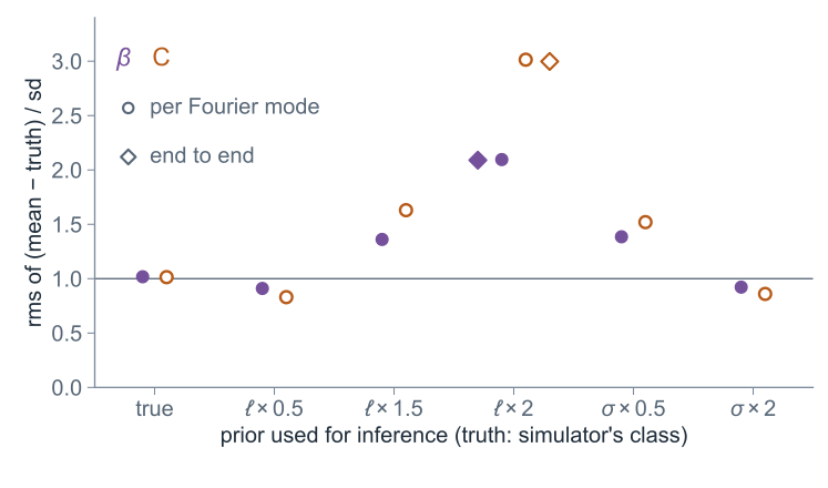
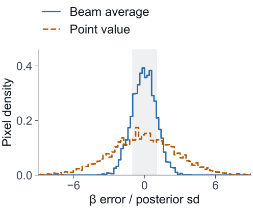
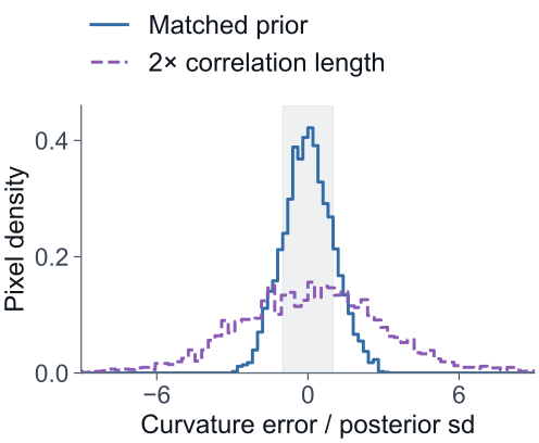
Correlation length 2× too long: z rms 2.10 (β) and 3.01 (C) per Fourier mode, 2.09 and 3.00 end to end. Not done: inferring the correlation length and amplitude.
beam-smoothed prior class · \(f=10^{-3}\) · dots: per Fourier mode, uniform one visit · diamonds: end to end, stripes and hole
[Backup; how much of the curvature map is data.] One pointing on its own fixes β to 2.6 × 10⁻³ and C only to 0.025, about the rms of the C field. The joint posterior is much tighter because the smoothness prior shares information between neighbouring pixels; for C most of the precision comes from the prior. That makes the prior the weak point. With the correct hyperparameters the z rms is 1.02 (β) and 1.01 (C); a correlation length too long by 1.5 or 2, or an amplitude half the truth, makes the intervals too narrow, and C suffers most: z rms 3.00 end to end for twice the length. Too short or too large a prior is conservative. The point-field prior, which ignores the beam smoothing, over-covers: 74% and 71% instead of 68; across 16 realisations its β z rms median is 0.89, which fails the pre-registered calibration check, so the slides use the beam-smoothed prior. A wrong prior class, as opposed to wrong hyperparameters, is untested. The next step is to infer the correlation length and amplitude with the maps.
Backup · Part 3 · Spectral maps · 16 realisations
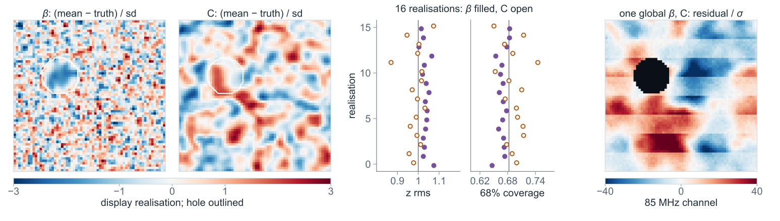
Errors against beam averages match the sd in 16 realisations
beam-smoothed prior · 16 realisations redraw the sky and the noise; posterior sd from the display realisation z rms (median), β / C 68% coverage (mean), β / C
observed pointings 1.03 / 0.99 67% / 69% hole 0.88 / 0.88 66% / 71%
[Backup; is the display realisation typical?] The 16 calibration realisations redraw the sky fields and the noise and keep the coverage, so the posterior covariance, and hence the sd map, is the same as for the display realisation; only the mean is recomputed. Against the beam averages the standardised errors have z rms near one and the 68 per cent intervals cover 67 to 69 per cent of observed pointings. In the hole there are only 183 pointings per realisation, so the hole numbers scatter more; their mean coverage is 66% for β and 71% for C. The right panel shows why a map is needed: one global β and C leaves residuals of 16.5 σ rms at the top channel.
Backup · Part 3 · A RHINO-sized chromatic beam
Infer the beam and the sky spectrum together
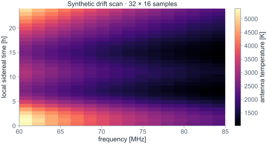
Synthetic ring drift scan · 96 sky pixels · 32 LST bins · 16 channels · 60–85 MHz
\[T(\phi,\nu)=A\,T_0(\phi)(\nu/70)^{-\beta}\]
\[w(\nu)=w_{70}(\nu/70)^{-0.8}\]
Known sky template, Gaussian beam.
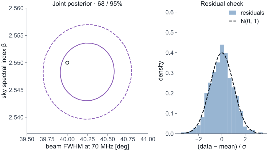
Inject \(w_{70}=40^\circ,\ \beta=2.55,\ A=1\).
One forward model: sky maps → chromatic beam → time–frequency data.
With a chromatic beam of RHINO's size, 40° at 70 MHz, the narrow-beam shortcut does not apply, so the beam stays in the forward model. Now put the method into a forward model. The sky is a synthetic ring and the beam a Gaussian; no RHINO beam measurement enters. Its known spatial template has a frequency power law with unknown beta, and the Gaussian beam has an unknown full width at half maximum at seventy MHz and a prescribed chromatic scaling, nu to the minus 0.8; the RHINO scaling quoted on the limits slide is 0.66. We free one common sky normalization and integrate it analytically. [Advance.] Inject a forty-degree beam and beta two-point-five-five with twenty-kelvin independent noise. [Advance.] The data on the right are generated by maintained Rheplicant MapSky, MatrixProjector and SkySourceOperator inside the Pipeline. The posterior uses its algebraically equivalent factorized forward, verified against that Pipeline. Only width and beta remain for a two-dimensional posterior grid. Spatial template, pointing, chromaticity and noise are fixed. This example contains no global 21-cm signal; a global-signal application would use an m-mode treatment. [Scope.] New synthetic calculation of 10 Oct 2026 with the maintained MapSky and MatrixProjector.
Backup · Part 3 · A RHINO-sized chromatic beam
The full drift scan constrains both unknowns
Same synthetic data and forward model · numbers: 801 × 801 grid, contours: 401 × 401 · shared amplitude integrated out
\(w_{70}=(40.25\pm0.22)^\circ\)
\(\beta=2.5483\pm0.0035\)
Posterior means ± standard deviations.
Joint correlation \(\rho=0.020\).
Check the entire posterior, then the predicted observation.
This is the joint posterior. Beam FWHM and spectral index are both recovered within their uncertainty in this realization; the ring is the injected truth. The quoted numbers are posterior means and standard deviations, conditional on the stated model. [Advance.] Their correlation is small with the whole drift scan. The residual distribution, after subtracting the posterior mean model, has rms close to one noise standard deviation. [Advance.] We doubled the grid, compared the factorized calculation against the actual Rheplicant forward, and independently integrated the normalization. These checks validate the computation for this realization. They do not establish coverage across noise realizations or real-data calibration. The next slide compares one LST with all 32. [Scope.] Fresh synthetic posterior; uniform priors: FWHM 25° to 55°, beta 2.45 to 2.65. The quoted numbers come from the 801 by 801 grid, the contours from the 401 by 401 grid.
Backup · Part 3 · A RHINO-sized chromatic beam
Time dependence separates beam width from spectral slope
Controlled comparison · same truth, noise law, priors and common amplitude
One LST at 0 h FWHM sd 8.6°, as in the 25°–55° prior.
All 32 LSTs FWHM sd 0.22°; \(\beta\) sd 0.0035.
Keep the angular modulation in the data: it constrains the beam while the spectrum constrains \(\beta\).
Hold the model and priors fixed, but use only the first time bin. The broad orange region is a ridge: changing the beam changes which part of the template contributes, and a spectral-index change compensates, beta rising by about 0.0021 per degree of FWHM. The FWHM marginal is the prior box: its sd, 8.6 degrees, is the sd of the uniform 25 to 55 degree prior, so one LST carries no FWHM information. The correlation of the two, 0.79, is set by the box as well. [Advance.] Use all thirty-two times and the purple posterior shrinks to a small spot, shown in the zoom inset; its full shape was on the previous slide. Its FWHM sd is 0.22 degrees, against the prior's 8.7. [Advance.] The inference works because the model predicts angular modulation as well as the spectrum. This result assumes known spatial sky structure and beam chromaticity. Relaxing them requires a larger model. [Scope.] Synthetic ring drift scan; contours at 68 and 95 per cent from the 401 by 401 grid; no real RHINO or CST beam measurement.
Backup · Part 3 · bayesmith · Basic methods
Gaussian structure makes inference tractable
bayesmith · exploit Gaussian blocks; correct to the full target
Solve, draw, integrate GLS, constrained realisations
Build a Gaussian proposal Iterative GLSGauss–Newton linearisation
Recover the full target Metropolis–Hastings correction
A non-Gaussian posterior can still be reached with Gaussian proposals
Many data models contain Gaussian blocks; the Hydra samplers on the previous slides rely on them. bayesmith collects the operations that use them. Exact Gaussian conditionals support a solve, a draw or analytic integration. [Advance.] When the dependence is nonlinear, moving-noise GLS, log-linearisation and Gauss–Newton construct Gaussian proposals. [Advance.] The proposal is corrected with Metropolis–Hastings or importance weights; NUTS remains available for general blocks. [Advance.] The Gaussian is the computational tool; the posterior can be strongly non-Gaussian. The next two examples infer population statistics from one bank of Gaussian draws, with 8 and 144 latent values. The methods are the eight of the inference notebook's methodology guide, grouped by their job.
Backup · Part 3 · bayesmith · Gaussian reference reweighting
Draw Gaussian fields, then weigh the non-Gaussian law
Observation: \(d=Rx+\epsilon\), Gaussian noise; population law \(p_\eta(x)\)
1 · One Gaussian reference posterior \(x_i\sim q(x\mid d)\propto p(d\mid x)\,p_0(x)\) · fast GCR draws
2 · Evaluate the complete field's density ratio \(w_i(\eta)=p_\eta(x_i)/p_0(x_i)\)
3 · Infer the population, then draw the field \(p(\eta\mid d)\propto p(\eta)\,\frac1N\sum_iw_i(\eta)\)
Draw \(\eta\); choose a whole \(x_i\) with its weights at that \(\eta\).
Fixed likelihood here. Check weight ESS and independent banks; the finite bank is an approximation.
Take a linear observation with Gaussian noise. Replace the population law by one convenient Gaussian reference and draw its conditional fields using GCR. [Advance.] For a proposed population hyperparameter, evaluate the non-Gaussian prior of each complete field divided by its reference prior. The likelihood is unchanged, so it cancels. [Advance.] The mean weight estimates the marginal likelihood ratio. Multiply by the hyperprior, normalise on a physical parameter grid, draw the hyperparameter, then draw a whole field using the weights at that value. This preserves the joint dependence. [Advance.] Check effective weight count and a fresh bank. This demo adds quadrature and joint resampling to PosteriorReweighting, whose fit API returns a marginal MAP. It does not turn finite importance sampling into an exact sampler or a missing-tail guarantee. Whole-field weights degrade as the field grows: the examples here have 8 and 144 latent values, and the backup Poisson sky at 16,384 coefficients needed its exact cell-by-cell factorisation. For local state-dependent Gaussian proposals the complementary method is MH, including the forward and reverse proposal densities.
Backup · Part 3 · bayesmith · Example 1 · Two populations
Infer a bimodal population with Gaussian field draws
\[d_j=x_j+\epsilon_j,\quad\sigma_\epsilon=0.35\]
\[\begin{aligned}p(x_j\mid a)={}&(1-a)\,\mathcal N(-1,0.6^2)\\&+a\,\mathcal N(1,0.6^2)\end{aligned}\]
Eight observed objects. Infer the mixture fraction \(a\sim\mathrm{Beta}(2,2)\).
Reference: \(p_0(x_j)=\mathcal N(0,1.5^2)\).
\(a\): 95% interval [0.28, 0.85]
Each observed object is a noisy latent value. That latent comes from either a population near minus one or a population near plus one; the unknown a is the fraction in the second population. Eight observations and a Beta two-two prior. The left panel shows the non-Gaussian law. [Advance.] Draw eight-dimensional fields from one Gaussian reference posterior; use their whole-field density ratios for a. [Advance.] The right panel shows the posterior of a: the two independent banks overlap the analytic mixture convolution. The interval is broad, as eight objects warrant. Four thousand joint field/population draws are stored, and the field draws depend on a. [If asked.] The ESS is the minimum over the central 99 per cent of a. Synthetic data; the check is the analytic Gaussian-mixture convolution.
Backup · Part 3 · bayesmith · Example 2 · Source counts
The Gaussian covariance stays fixed; infer the skewness
Synthetic 12 × 12 grid · prior λ ~ U(0.5, 8)
\[n_j\sim\mathrm{Poisson}(\lambda)\]
\[x_j=\sqrt{0.8/\lambda}(n_j-\lambda)+g_j\]
\(g_j\sim\mathcal N(0,0.2)\); observe \(d=B(x+\epsilon)\).
\(K_1=0,\ K_2=1\) at every \(\lambda\).
\(\lambda>0.78\) at 97.5%, so \(K_3<0.81\)
The model is source counting. Draw a Poisson number of sources in each cell, subtract the mean, scale its amplitude, and add a diffuse Gaussian field. A known beam blurs the sky and the noise together; the noise is white before the beam. The toy beam can be inverted, so no information is discarded. [Advance.] Changing the rate keeps the mean and covariance fixed and changes the skewness and the fourth cumulant. A Gaussian likelihood for those statistics alone cannot measure the rate. A Gaussian posterior bank plus the full Poisson-Gaussian density ratio can. [Advance.] Two banks agree with the analytic convolution. The data set the lower end: the rate is above 0.78 at 97.5 per cent, so the skewness K3 is below 0.81. The upper end is the prior's. As the rate grows the model tends to a Gaussian with the same covariance, so the likelihood levels off; at the bound, rate 8, the posterior density is still 4 per cent of its peak. Zero skewness, the Gaussian limit, has a likelihood e to the minus 6.2 of the maximum. [If asked.] With the bound at 16, 32 or 64 instead of 8, the upper end moves to 0.86 to 0.89 of the bound, while the lower end stays between 0.78 and 0.81. The prior on the rate is uniform from 0.5 to 8. The diffuse variance is 0.2 and the noise sd 0.1; the count cutoff 48 was checked against 96. The weights use complete 144-cell fields. Whole-field weights degrade as the field grows; the backup Poisson sky at 16,384 coefficients needed its cell-by-cell factorisation.
Backup · Part 3 · Bayesian analysis at scale · From population examples to an instrument
One model graph holds a sky and an instrument
Forward simulation Draw parameters → generate a measurement.
Bayesian inference Condition on the measurement → infer parameters. Same arrows, same physical calculation.
[From the population examples to the sky.] The two examples had a population law over one field. A real experiment is one hierarchical model with the sky and the instrument inside it: population hyperparameters govern sky parameters; physical sky components, the moment basis of part two among them, feed an instrument response with its own uncertain parameters; a noise model turns the prediction into a probability for the data. Every box is a differentiable function, so the graph is read forwards, draw and simulate, [advance] or backwards, condition on data and infer; bayesmith assigns each block of unknowns a method. The physics is the same in both directions. What is missing is the instrument box. [If asked.] Each box can itself be a graph of differentiable operators.
Backup · Part 3 · rheplicant + bayesmith · A synthetic narrow-beam survey
Logs turn a curved power-law sky into one Gaussian block
Synthetic periodic patch · 64 × 64 pointings · 16 channels, 60–85 MHz · narrow achromatic beam, not RHINO's
Simulated with rheplicant: 256² sky
\[\ln T_q=t_q-\beta_qL+C_qL^2\]
\[d_p=\textstyle\sum_q B_{pq}T_q\,(1+f_p w)\]
\(L=\ln(\nu/70\,\mathrm{MHz})\); beam 1.5 pointings; \(f_p=10^{-3}\) for one visit, \(5\times10^{-4}\) for four; one hole.
Inferred: one spectrum per pointing
\[\ln d_p=t_p-\beta_pL+C_pL^2+f_p w\]
Linear in \(t,\beta,C\); noise \(f_p\) in every channel.
Gaussian-field priors on \(\beta\) and \(C\): 12,288 unknowns, 62,608 data, one Gaussian block, exact independent draws.
one global β, C: χ²/dof = 123
[From twin to resolved sky.] Give the sky box three slides back a spectral index and a curvature in every direction. RHINO's forty-degree beam cannot resolve those maps; a narrow-beam survey can. So I simulate one with rheplicant: a sky four times finer than the pointings, a curved power law in every pixel, a beam of 1.5 pointings, noise of one part in a thousand per channel, and one unobserved hole. [Advance.] The inference model takes the log of each pointing's spectrum. The noise becomes additive and the curved power law a quadratic in L. On the right, two pointings with the fitted power law removed. [Advance.] Gaussian-field priors on β and C make it one linear-Gaussian block of 12,288 unknowns, which bayesmith draws from exactly. [Advance.] Why maps: one global β and C gives χ² per degree of freedom of 123; β and C per pointing give 0.99. [If asked.] The sky box is the graph's map-based foreground. The simulator applies the beam in temperature; the noise is radiometer noise for one visit, and four visits halve it. The log turns multiplicative noise into additive noise of width f, after a known shift of f squared over two. f = 10⁻³ is a 0.64 s visit in 1.56 MHz channels. The two pointings follow a fixed rule: the four-visit pointing with the largest posterior-mean |C| and the one-visit pointing with the smallest; their error bars are in log space. The prior describes the beam-smoothed field, the field the data measure. bayesmith's factor_partition finds the log block; compile() does not choose that route for this graph yet, so the draws call log_linear_operator and a jitted gcr_sample. The route table is in backup.
Backup · Part 3 · rheplicant + bayesmith · Synthetic survey · Posterior maps
Exact draws map β and curvature; their errors follow the scan
12,288 unknowns: 1.3 s per independent draw; CG error ≤ 0.01 sd in every pixel of every draw
[Let the maps sit.] Top row the spectral index at 70 MHz, bottom row the curvature; left the truth, right the posterior mean. The truth is the beam average the data measure; the next slide says why. [Advance.] The posterior standard deviation follows the scan: stripes where it passed once or four times, and the hole, where only the neighbours and the prior constrain the map. [Advance.] A cut through the hole: the truth in white, five independent posterior draws, and the two-sigma band from 200 draws. Outside the hole the draws sit on the truth; inside they spread. Each draw is a whole map of 12,288 numbers. [Advance.] A draw takes 1.3 seconds and does not depend on the previous one: no chain and no burn-in. Its solver error is certified below a hundredth of a posterior standard deviation in every pixel. At 432 unknowns with the same scan pattern an exact draw takes 23 milliseconds. NUTS took 3 minutes per chain for a thousand draws after a thousand warm-up steps and had not converged: the two chains disagree, R-hat up to 1.092 for a β pixel, and one chain has as few as 14 effective draws for a curvature pixel. 12,288 sits on the ladder of slide 31, between the drift scan and the 21-cm cube. [If asked.] The truth is weighted by the sky brightness. For β the posterior sd is about 1.2 × 10⁻³ in single-visit stripes, 7.4 × 10⁻⁴ in four-visit stripes and 1.0 × 10⁻² in the hole. Where NUTS converged, its posterior means differ from the exact draws by at most 0.12 NUTS standard deviations in uniform coverage at 432 unknowns (two chains, R-hat at most 1.01) and by at most 0.15 at 108 unknowns (means and sds pooled over two chains, R-hat at most 1.01, at least 983 effective draws per chain). In the stripes 82 of the 144 curvature pixels have R-hat above 1.01. The NUTS cost per effective draw is the wall time of one chain, compilation and warm-up included, over its smallest effective sample size among the β and C pixels: 0.84–0.89 seconds in uniform coverage, and 11–13 seconds in the scan stripes, where the effective sample sizes come from unconverged chains. NUTS was not run at 12,288. At this size a dense Cholesky factorisation, with t eliminated pointing by pointing, also draws exactly: 1.5 seconds to build, factorise and solve for the mean, then 0.3 milliseconds per draw, so here it is faster for more than one draw. It is the check in the backup. Its memory grows as the square of the number of unknowns and its cost as the cube; the conjugate-gradient route needs only applications of the operator. The solver bound uses the residual and the prior: in whitened coordinates the posterior precision is at least the identity, so the residual norm bounds the error of every pixel in units of its posterior standard deviation. The relative error of the whole vector is certified below 5.0 × 10⁻⁴, with the largest eigenvalue bounded analytically; bayesmith's default twelve-step estimate of that eigenvalue is 0.6 per cent low on this operator. Per pixel, the data alone fix C only to 0.025, about the rms of the C field itself (0.025). The joint posterior reaches 0.0036 in single-visit stripes because the smoothness prior shares information between pixels, so the curvature map leans on the prior; the next slide shows what a wrong prior does. The cut was fixed through the hole centre before plotting. Along it the curvature truth leaves the two-sigma band at 3 of 64 pointings, 1 of them in the hole; over 16 realisations the 68 per cent intervals in the hole cover 66% (β) and 71% (C). Timings were taken on an Apple M3 Ultra with other jobs running (one-minute load 2.1 to 8.4); the NUTS chains were rerun one at a time, at load 1.8 to 3.2.
Backup · Part 3 · Model → plan → inference
A good fit can still give the wrong map.
Beam-averaged sky Know which sky the map estimates.
Chromatic response A good residual can hide a biased map.
Prior smoothness Smoothness changes the uncertainty.
Here the same saved survey tests three modelling choices. The blue histogram measures beta against its brightness-weighted beam average; the orange one measures it against the point value. We must name which sky our map estimates. [Advance.] This error map comes from making the beam chromatic while retaining the achromatic log inference model. The spectral residual still looks statistically normal, but beta is biased. [Advance.] Doubling the prior correlation length broadens the curvature error distribution in units of the reported uncertainty. Fast sampling does not remove the need to check the physical model. [If asked.] Histograms use observed pixels, with densities normalised over all values; the visible tails are cropped without renormalisation. Pixels are correlated, not independent coverage trials. The pale band is plus or minus one posterior standard deviation. The matched beta rms error is 1.03 sd; against point values it is 2.95 sd. The chromatic stress test gives 39.18 sd beta rms bias with chi-square/dof 0.993. Prior length twice the generating class gives curvature rms error 3.00 sd and 27.4 percent pointwise coverage of the nominal one-sd band. These are full-run results for this synthetic patch, not a general calibration guarantee. No noise-free prediction curves are used. [Archived technical qualifications.] [What the maps measure; where the method stops.] Through a beam, a log-quadratic fit does not return the index under the beam centre. Its slope is the brightness-weighted beam average of β; its curvature is the average C plus half the variance of β inside the beam: the truths of the previous slide. [Panel.] Each point is a full run; the axis is beam width over the coherence length of β. Against beam averages the error stays near one; against point values it grows with the width. The model fits at any width; the width decides what β means. [Advance.] A beam whose width scales as ν to the minus 0.66, as RHINO's does, mixes angular structure into the spectrum: 39 sigma in β, while χ² per degree of freedom stays 0.99. For RHINO the beam stays in the forward model. [Advance.] At f ≥ 0.06 bayesmith refuses the log step; at f = 10⁻⁴ unpreconditioned conjugate gradients no longer certify the draw. A prior correlation length twice too long gives curvature errors of 3.0 posterior sd rms. [Only if the room is with you.] The half-variance term is part two's moment expansion: averaging power laws produces curvature, and here the population is the sky inside the beam. [If asked.] The weights are the beam times the sky brightness at 70 MHz. Against them the 68 per cent intervals hold the truth in 67% (β) and 68% (C) of the observed pixels. RHINO's beam narrows from 44 to 35 degrees across the band, the same inference model is used for the chromatic run, and the backup shows a RHINO-sized beam inside the forward model. f = 10⁻⁴ is about a minute per visit. Against point values the β error is 3.0 sigma rms at this beam and 169 sigma at twice the coherence length. The multiple depends on the prior: at that width the beam-smoothed prior gives a median β sd of 2.3 × 10⁻⁴ and the point-field prior 1.6 × 10⁻³, so with the point-field prior the same error is 29 sigma. The error itself, 0.034 rms in β, is the same under both priors. Against beam averages the z rms stays between 1.0 and 1.2 at every width tested. Over 16 realisations the mean coverage is 67% (β) and 69% (C). In noise-free fits a beam five times narrower lowers the spurious chromatic β only from 0.066 to 0.051 rms. At 108 unknowns and f = 0.001, 0.03, 0.0599, the posterior means of the log step lie within 0.15 NUTS standard deviations of NUTS on the original likelihood, with sd ratios 0.976–1.001; the NUTS means and sds are pooled over two chains with R-hat at most 1.01. At 3 × 10⁻⁴ conjugate gradients still certify the draw. The prior result comes from the display realisation, with 27% coverage. Each run on this slide uses one sky and noise realisation, one coverage pattern on a periodic flat patch and a prior of the simulator's class; the 16-realisation check is in backup. A sum of components, including a 21-cm signal, is not log-linear; logs linearise one dominant component. A noise-free prediction of these errors, the posterior mean of noise-free data plus the noise variance of that mean, differs from the full runs by up to 3.5 per cent against point values and 10.3 per cent against beam averages. The limit set before the run was 10 per cent, so the panel shows full runs only. For the worst case the run-to-run scatter of that number over 200 noise realisations is 11 per cent.
Backup · Bayesmith example
A real model. An automatically generated sweep.
Traced synthetic model · known design inputs omitted · coloured parameters identify the two updates
Random field + background Moving-noise GLS proposal + MH
Power + shape + gain + noise NumPyro NUTS · conditional on the field
These are the notebook’s actual generating components, and below them their traced model. A power spectrum generates a random Fourier field; a known response acts on it. We add a nonlinear bump and background, multiply by a gain, then observe with signal-dependent noise. [Advance.] The returned plan groups the field and background into one update using a moving-noise GLS proposal, corrected by Metropolis–Hastings against the declared target. [Advance.] Power, nonlinear shape, gain and noise form the NUTS remainder. Each update conditions on the current value of the other block. This is the reusable part of the design: the scientist writes the model; the compiler returns the sweep. [If asked.] Demo 06 composed_process, automatic proposal selection, fourteen coordinates in the first block and six in the remainder. Nodes and edges are from its saved result.json, laid out with the notebook’s own dag_svg renderer. Five constant/design nodes are omitted; all displayed dependencies remain intact. These are proposal-based updates, not exact untruncated GCR. The numerical evidence is the existing verified run; no new inference was run for this edit.
Backup · Bayesmith example
Approximate the update. Keep the model.
Structured proposal + original-target MH · nonlinear remainder sampled by NumPyro
The same model now predicts the observed signal. Orange dashed lines show the generating mean; the blue interval is the ninety-nine per cent posterior interval for the mean signal. The lower plot shows data minus the fitted mean. [Advance.] These are two saved parameter posteriors. The shape location is tightly measured, while one process realization gives a broader power-scale posterior. The proposal exploits an easier local problem. MH evaluates the original target and the forward and reverse proposal densities, retaining the declared priors and support. The remaining parameters are handled by the backend. [If asked.] Every eighth observation is plotted for legibility; the run used all 3,840. Purple histograms show saved samples, not a new experiment. One simulated dataset demonstrates this workflow; it is not a coverage or efficiency benchmark. The verified run used two chains; R-hat was at most 1.0087, minimum ESS 672, no divergences. These diagnostics belong only to this notebook case. Bounded GLS proposals are approximate; target correction does not by itself establish finite-run convergence. Dashed truth lines apply to both posterior panels.
Discussion · Observation and inference
Examples and further directions
Open only the example relevant to the audience's question. These are the former main38–44 examples, with their saved figures and qualifications. They are separate demonstrations, not a single verified end-to-end pipeline.
Backup · Part 3 · Bayesian analysis at scale · RHINO
RHINO: an observing system to model
Jodrell Bank · photo P. Bull Sky-averaged 21-cm signal Sky and instrument response Reference measurements Calibration uncertainty inside the model
RHINO is one observing system that motivates this approach: a radio experiment aimed at the sky-averaged21-cm signal. The scientific inference has to connect a sky model to actual measurements. [Advance.] Those measurements depend on both the sky and the instrument response. [Advance.] Reference measurements add calibration information. [Advance.] We want their uncertainty inside the same observation model, so it can be carried into the inference. The next diagram shows how Rheplicant composes those pieces. The demonstrations that follow use synthetic observations. [If asked; system details.] [Keep the claims modest.] RHINO's design is a 7.2 by 6.0 metre pyramidal horn aimed at the sky-averaged 21-cm signal between sixty and eighty-five megahertz, led by Phil Bull at Manchester: directive and well defined, which is why a horn, and chromatic, which is why it needs a model. At Jodrell Bank a scaled 350 MHz prototype is under construction. [Advance.] The receiver switches between the antenna and two thermally stabilised loads, with an in-situ vector network analyser and a continuous-wave tone for gain tracking; [advance] the noise-wave temperatures must be known to a tenth of a kelvin under a sky of a few thousand kelvin. Nothing on the sky yet; everything that follows is on simulated nights. [If asked.] Table 1 of the paper gives the 7.2 by 6.0 metre aperture and the 44 to 35 degree beam; the loads sit near 380 and 490 K.
Backup · Part 3 · Model → plan → inference
Rheplicant draws the twin it assembles.
Sky → antenna Switch → receiver Readout Native tour assembly · ⊕ adds branches · the diamond switches between antenna and reference loads · loads ×3
This is the package’s own signal-path rendering, the same output embedded by rheplicant-agent. The left view adds foreground and global signal, applies the horizon split and antenna loss. [Advance.] The native switch connects the antenna or one of three reference loads; noise-wave response and bandpass belong downstream. [Advance.] Gain, thermal noise and digitisation produce the raw readout. These are the operators in the documentation tour’s actual assembled twin. The stages are reusable objects in an executable calculation. [If asked.] These three views retain native shapes, colours and lit state. The same boundary operator is repeated across neighbouring views to orient the reader. Identity-only stretches and unused branches are omitted; every contracted edge’s full template path is saved in provenance. The unmodified Assembly.to_svg graph is linked below. The tour uses an analytic foreground and a horizon split, not the synthetic narrow-beam example in the main talk. [A software slide: the name, the link, what it is.] rheplicant, a replica of an antenna, is RHINO's digital twin: one pure JAX function from sky and instrument parameters to raw data. Sky through the beam, horizon and ground, ohmic loss, mismatch, switched loads and receiver noise waves, every stage differentiable, so the twin that simulates an observation also calibrates it. [Advance.] Four things it does on the same object: simulate forwards, infer backwards, replace a stage by a neural surrogate, and keep a campaign as streamed evidence. [Advance.] The second and the fourth run on bayesmith, which has no radio astronomy in it; rheplicant holds what depends on the instrument and calls bayesmith for the arithmetic that does not. [If asked.] JAX and Equinox; State and Operator are the two nouns, cascade, sum and switch the three combinators; a 33-node canonical signal path; seventeen of twenty-nine radio operators are documented placeholders and the run record says so; 12,200 tests.
Backup · Part 3 · Model → plan → inference
Larger maps. The same inference machinery.
One joint field update Keep the map’s spatial structure.
Independent map draws Reuse the Gaussian update.
Numerical accuracy checked Check the solve as the field grows.
Reuse the method as the field grows.
The benefit is a reusable inference method. This saved benchmark increases the size of a joint Gaussian field while keeping the same update machinery. Each point measures the time for an independent draw of the full field. [Advance.] We do not design a new sampler at each map size: the supported Gaussian structure lets us reuse the field update. [Advance.] The numerical solve is checked as the field grows. This is the ambition of Bayesmith: make inference design reusable, so scientists can spend more time on the model. [If asked.] The six saved operator/model-generated Gaussian benchmarks have108,432,768,3072,12288 and49152 latent coordinates. Median seconds per independent draw are0.00470,0.02355,0.04332,0.23610,1.32184 and8.11241, measured on an Apple M3 Ultra. These points do not each rerun the complete observation pipeline; full end-to-end runs and solver certificate scopes are in backup. The curve does not claim linear scaling, universal speedup, arbitrary-DAG efficiency or general automatic route selection. GCR is an independent conditional draw for an eligible Gaussian block; other blocks can require corrected proposals or a numerical backend. Physical-model checks remain necessary and are retained in backup.
Backup · Part 3 · Model → plan → inference
Tools for agents. Results you can inspect.
rheplicant-agent / Workbench Flagging rounds · recorded tool executions
First tool call Refined result · checks repeated Four fixed checks · every call Call Stable Residual Protected Complete Verdict 1First pass — ✓ ✓ — continue 2Refine ✓ ✓ ✓ — continue 3Broaden — ✓ ✓ ✓ continue 4Repeat ✓ ✓ ✓ ✓ pass
Stop when every fixed check passes.
Here is a different capability: make observation tools available to agents, with results we can inspect. This recorded synthetic example flags contaminated samples; orange marks show the tool’s output. [Advance.] Each call leaves a record and runs the same fixed checks. We can see what changed, which checks passed, and why another call is needed. [Advance.] The final repeat passes every check, so the procedure stops. The vision is an agent that works through executable tools, with decisions grounded in their returned results. [If asked.] The table is an enlarged transcription of the Workbench’s actual four-round timeline; masks are the exact published boolean arrays, not block-averaged occupancy. These are recorded real rheplicant_flag executions driven by a scripted sequence, replayed in a seeded session; no live language model ran this demonstration. The plugin makes the same tools and guidance available to an agent. Mask fractions are 3.22, 3.34, 4.57 and 4.57 percent; occupancy changes are unknown in the first round, then 0.122, 1.22 and zero percentage points. Protected channels remain clean in all four calls. The RFI and noise operators in this synthetic fixture have placeholder physics; passing these operational checks is not scientific validation of real RFI removal. Broad kernels are 3 by 3 and 1 by 9; residual check uses excess kurtosis. The actual UI, waterfall and chat replay remain in backup.
Backup · Part 3 · Model → plan → inference
Keep learning as observations arrive.
Night 1 + Night 2 + Night 3 Top: new data (dots), generating mean (orange) · bottom: 95% joint posterior · +: truth · dashed: earlier nights
Stored information reproduces the full-data posterior.
One final capability is to carry information forward through an observing campaign. New data arrive each night; the lower plot shows what we have learned about the shared signal and foreground parameters. [Advance.] Night two adds information to the same inference. [Advance.] Night three adds more; the dashed contours keep the earlier results visible. In this example, the stored likelihood information reproduces the posterior from all the original samples. The vision is a campaign that keeps learning as observations arrive, even after recordings are archived. [If asked.] This is a newly checked synthetic three-night example using the current Rheplicant compress_linear and BayesMemory APIs. The trough location 72 MHz and width 4.5 MHz are fixed; global amplitude and foreground tilt enter affinely. Tilt is the Kelvin coefficient of the dimensionless frequency coordinate (frequency minus 72 MHz)/12.5 MHz, internally named slope. Independent nightly Gaussian offsets with sd 0.15 K are analytically integrated out; fixed Gaussian noise sd 0.22, 0.18, 0.16 K. The plotted spectra have a known nominal foreground removed; they are not real RHINO observations. There are 64 channels per night. Each lower contour is 95 percent probability for the joint two-dimensional Gaussian, not a one-dimensional95 percent interval. The global prior is applied once. An independent NumPy dense covariance calculation from raw data checks the normalised likelihood, means and covariance; reverse ordering and a save/load roundtrip are also verified. Exact compression here requires this affine-Gaussian structure and conditional independence; general nonlinear cases need separately validated reduced-basis approximations. The Python evidence layer is implemented; the campaign YAML section remains reserved. No arbitrary observation graph is claimed exactly compressible.
Backup · Further directions
What comes next
Lensing fold the Jacobi map, reduced shear and the source sample as external insertions; converged nonlinear bispectrum; ray-tracing validation
Synchrotron the moment foreground inside the twin with Faraday depth and polarisation; coverage over noise realisations; the chromatic stress band
Inference RHINO calibration on real data; live agent sessions on real nights; streamed campaign evidence; certificates for Gibbs sweeps; a preconditioner for long integrations; chromatic beams inside the forward model
↘ Technical backup
[Backup; optional extensions.] Next steps follow the same map. In lensing, fold the Jacobi map, the reduced shear and the source sample as external insertions, with a converged nonlinear bispectrum and ray-tracing validation. In synchrotron, extend the moment foreground inside the twin to Faraday depth and polarisation, check its coverage over noise realisations, and face the chromatic stress band. In inference, calibrate RHINO on real data, run the agent live on real nights, stream the campaign evidence, extend the certificates to Gibbs sweeps, add a preconditioner for long integrations, and put chromatic beams inside the forward model of the spectral maps.
Backup · Sources
Selected sources and implementation
Radio: Zhang & Chluba, A statistical framework for synchrotron emission , in prep.; SyncMoments 0.4.0. Bull et al. (2025), RASTI, RHINO. rheplicant 0.9 and bayesmith 0.10 on PyPI; Zhang (2025) MomentEmu, arXiv:2507.02179.
Gibbs sampling: Wandelt, Larson & Lakshminarayanan (2004), PRD 70, 083511; Eriksen et al. (2004), ApJS 155, 227; Eriksen et al. (2008), ApJ 676, 10; BeyondPlanck Collaboration (2023), A&A 675, A1; Galloway et al. (2023), A&A 675, A3; Kennedy et al. (2023), ApJS 266, 23; Murphy et al. (2026), MNRAS 551, 1503; Dutta et al. (2026), arXiv:2604.26885; Zhang, Bull, Santos & Nasirudin (2026), RASTI, hydra-tod. Foreground targets: Pritchard & Loeb (2012); Fixsen et al. (2011); Dowell & Taylor (2018); Chluba (2016); Abitbol et al. (2017); BICEP/Keck (2021); Irfan et al. (2023). Gibbs schematic after K. Glasscock, RHINO overview (P. Bull).
Formalism: Zhang, Bull, Clarkson & Nicola, Statistical Field Theory for Weak Gravitational Lensing , arXiv:2606.19472, and its analysis package. Software: sft-wick, arXiv:2606.19480; kappa_PDF for the controlled optical PDF models; Unify-WL for the correction panorama.
Stochastic optics: Fleury, Larena & Uzan (2015) . Precision shear modelling: Euclid Collaboration (2024) . Source sampling and finite images: lensing bias , extended sources .
PDFs: Patton et al. ; Clerkin et al. ; Barthelemy et al. ; Zhong et al.
Provenance and hashes: assets/source_manifest.json · generated_manifest.json · reused_manifest.json · SOURCES.md
These are the sources supporting the main claims. The local source ledger identifies the manuscript, package and saved products used for each figure. Figures reused from the earlier talks are byte-identical copies, and the withdrawn FK B/E and redshift-sweep plots are not shown anywhere.