Joint Bayesian calibration and map-making for intensity mapping experiments Zheng Zhang Jodrell Bank Centre for Astrophysics, Department of Physics University of Manchester Manchester, UK JBCA Colloquium, Manchester, 28 May 2025
What this talk is not Not an end-to-end Bayesian model - by design Reasons • Component separation is not necessary/essential for gain/noise calibration • No reliable ground-truth sky model → model dependence becomes a liability Not: “We model this way to minimise degeneracy ” Instead • Model degeneracies when they exist • Model ignorance with general, safe representations • Stay true to what we exactly know 1. Introduction 1.1. What this work is (not) 2/20
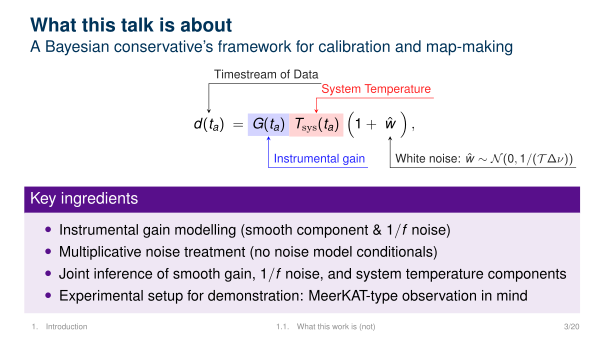
What this talk is about A Bayesian conservative’s framework for calibration and map-making d(ta) = G(ta) Tsys(ta) ( 1 + ˆw ) , Timestream of Data Instrumental gain System T emperature White noise: ˆw ∼ N (0, 1/(T ∆ν)) Key ingredients • Instrumental gain modelling (smooth component & 1 /f noise) • Multiplicative noise treatment (no noise model conditionals) • Joint inference of smooth gain, 1 /f noise, and system temperature components • Experimental setup for demonstration: MeerKA T -type observation in mind 1. Introduction 1.1. What this work is (not) 3/20
Instrumental Gain Modelling G(ta) = g(ta) (1 + ˆϵ ) Smooth gain 1/f noise (stochastic fractional gain) Flicker Noise Pˆϵ(f ) = { 0, |f | < fc, (f0/|f |)α , |f | ≥ fc. g(ta) = 4∑ n=0 an Pn(x), x = 2(ta − tmin) tmax − tmin − 1. 0 200 400 600 800 1000 Time [s] 0.0003 0.0002 0.0001 0.0000 0.0001 0.0002 Fractional Gain Error 1/f vs Time 2. Data Model 2.1. Smooth Gain 4/20
Stochastic Gain Model G(ta) = g(ta) (1 + ˆϵ ) Smooth gain 1/f noise (stochastic fractional gain) Flicker Noise (Complete Model) Gaussianity and stationarity . Pˆϵ(f ) = { 0, |f | < fc, (f0/|f |)α , |f | ≥ fc. g(ta) = 4∑ n=0 an Pn(x), x = 2(ta − tmin) tmax − tmin − 1. 0 200 400 600 800 1000 Time [s] 0.0003 0.0002 0.0001 0.0000 0.0001 0.0002 Fractional Gain Error 1/f vs Time 2. Data Model 2.2. Stochastic Gain 5/20
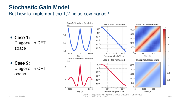
Stochastic Gain Model But how to implement the 1 /f noise covariance? • Case 1: Diagonal in DFT space • Case 2: Diagonal in CFT space /uni00000010/uni00000018/uni00000013/uni00000013/uni00000013/uni00000013/uni00000018/uni00000013/uni00000013/uni00000013 /uni0000002f/uni00000044/uni0000004a/uni00000003/uni0000000b/uni00000056/uni0000000c /uni00000010/uni00000013/uni00000011/uni00000018 /uni00000013/uni00000011/uni00000013 /uni00000013/uni00000011/uni00000018 /uni00000014/uni00000011/uni00000013 /uni00000014/uni00000048/uni00000010/uni0000001a /uni00000026/uni00000044/uni00000056/uni00000048/uni00000003/uni00000014/uni0000001d/uni00000003/uni00000037/uni0000004c/uni00000050/uni00000048/uni00000010/uni00000057/uni0000004c/uni00000050/uni00000048/uni00000003/uni00000026/uni00000052/uni00000055/uni00000055/uni00000048/uni0000004f/uni00000044/uni00000057/uni0000004c/uni00000052/uni00000051 /uni00000014/uni00000013/uni00000016 /uni00000014/uni00000013/uni00000015 /uni00000014/uni00000013/uni00000014 /uni00000029/uni00000055/uni00000048/uni00000054/uni00000058/uni00000048/uni00000051/uni00000046/uni0000005c/uni00000003/uni0000000b/uni00000026/uni0000005c/uni00000046/uni0000004f/uni00000048/uni00000012/uni00000037/uni0000004c/uni00000050/uni00000048/uni0000000c /uni00000014/uni00000013/uni00000017 /uni00000014/uni00000013/uni00000016 /uni00000014/uni00000013/uni00000015 /uni00000014/uni00000013/uni00000014 /uni00000014/uni00000013/uni00000013 /uni00000014/uni00000013/uni00000014 /uni00000026/uni00000044/uni00000056/uni00000048/uni00000003/uni00000014/uni0000001d/uni00000003/uni00000033/uni00000036/uni00000027/uni00000003/uni0000000b/uni00000051/uni00000052/uni00000055/uni00000050/uni00000044/uni0000004f/uni0000004c/uni00000056/uni00000048/uni00000047/uni0000000c /uni00000013/uni00000015/uni00000013/uni00000013/uni00000013/uni00000017/uni00000013/uni00000013/uni00000013 /uni00000037/uni0000004c/uni00000050/uni00000048/uni00000003/uni0000000b/uni00000056/uni0000000c /uni00000013 /uni00000014/uni00000013/uni00000013/uni00000013 /uni00000015/uni00000013/uni00000013/uni00000013 /uni00000016/uni00000013/uni00000013/uni00000013 /uni00000017/uni00000013/uni00000013/uni00000013 /uni00000018/uni00000013/uni00000013/uni00000013 /uni00000026/uni00000044/uni00000056/uni00000048/uni00000003/uni00000014/uni0000001d/uni00000003/uni00000026/uni00000052/uni00000059/uni00000044/uni00000055/uni0000004c/uni00000044/uni00000051/uni00000046/uni00000048/uni00000003/uni00000030/uni00000044/uni00000057/uni00000055/uni0000004c/uni0000005b /uni00000010/uni00000018/uni00000013/uni00000013/uni00000013/uni00000013/uni00000018/uni00000013/uni00000013/uni00000013 /uni0000002f/uni00000044/uni0000004a/uni00000003/uni0000000b/uni00000056/uni0000000c /uni00000010/uni00000015 /uni00000013 /uni00000015 /uni00000017 /uni00000014/uni00000048/uni00000010/uni0000001b /uni00000026/uni00000044/uni00000056/uni00000048/uni00000003/uni00000015/uni0000001d/uni00000003/uni00000037/uni0000004c/uni00000050/uni00000048/uni00000010/uni00000057/uni0000004c/uni00000050/uni00000048/uni00000003/uni00000026/uni00000052/uni00000055/uni00000055/uni00000048/uni0000004f/uni00000044/uni00000057/uni0000004c/uni00000052/uni00000051 /uni00000014/uni00000013/uni00000016 /uni00000014/uni00000013/uni00000015 /uni00000014/uni00000013/uni00000014 /uni00000029/uni00000055/uni00000048/uni00000054/uni00000058/uni00000048/uni00000051/uni00000046/uni0000005c/uni00000003/uni0000000b/uni00000026/uni0000005c/uni00000046/uni0000004f/uni00000048/uni00000012/uni00000037/uni0000004c/uni00000050/uni00000048/uni0000000c /uni00000014/uni00000013/uni00000017 /uni00000014/uni00000013/uni00000016 /uni00000014/uni00000013/uni00000015 /uni00000014/uni00000013/uni00000014 /uni00000014/uni00000013/uni00000013 /uni00000014/uni00000013/uni00000014 /uni00000026/uni00000044/uni00000056/uni00000048/uni00000003/uni00000015/uni0000001d/uni00000003/uni00000033/uni00000036/uni00000027/uni00000003/uni0000000b/uni00000051/uni00000052/uni00000055/uni00000050/uni00000044/uni0000004f/uni0000004c/uni00000056/uni00000048/uni00000047/uni0000000c /uni00000013/uni00000015/uni00000013/uni00000013/uni00000013/uni00000017/uni00000013/uni00000013/uni00000013 /uni00000037/uni0000004c/uni00000050/uni00000048/uni00000003/uni0000000b/uni00000056/uni0000000c /uni00000013 /uni00000014/uni00000013/uni00000013/uni00000013 /uni00000015/uni00000013/uni00000013/uni00000013 /uni00000016/uni00000013/uni00000013/uni00000013 /uni00000017/uni00000013/uni00000013/uni00000013 /uni00000018/uni00000013/uni00000013/uni00000013 /uni00000026/uni00000044/uni00000056/uni00000048/uni00000003/uni00000015/uni0000001d/uni00000003/uni00000026/uni00000052/uni00000059/uni00000044/uni00000055/uni0000004c/uni00000044/uni00000051/uni00000046/uni00000048/uni00000003/uni00000030/uni00000044/uni00000057/uni00000055/uni0000004c/uni0000005b /uni00000010/uni00000013/uni00000011/uni00000017 /uni00000010/uni00000013/uni00000011/uni00000015 /uni00000013/uni00000011/uni00000013 /uni00000013/uni00000011/uni00000015 /uni00000013/uni00000011/uni00000017 /uni00000013/uni00000011/uni00000019 /uni00000013/uni00000011/uni0000001b /uni00000014/uni00000011/uni00000013 /uni00000014/uni00000048/uni00000010/uni0000001a /uni00000026/uni00000044/uni00000056/uni00000048/uni00000003/uni00000014/uni0000001d/uni00000003/uni00000027/uni0000004c/uni00000044/uni0000004a/uni00000052/uni00000051/uni00000044/uni0000004f/uni00000003/uni0000004c/uni00000051/uni00000003/uni00000029/uni00000029/uni00000037/uni00000003/uni00000056/uni00000053/uni00000044/uni00000046/uni00000048/uni0000001e/uni00000003/uni00000026/uni00000044/uni00000056/uni00000048/uni00000003/uni00000015/uni0000001d/uni00000003/uni00000027/uni0000004c/uni00000044/uni0000004a/uni00000052/uni00000051/uni00000044/uni0000004f/uni00000003/uni0000004c/uni00000051/uni00000003/uni00000026/uni00000029/uni00000037/uni00000003/uni00000056/uni00000053/uni00000044/uni00000046/uni00000048 2. Data Model 2.2. Stochastic Gain 6/20
Stochastic Gain Model But how to implement the 1 /f noise modelling? • Case 2: Diagonal in CFT space (Ncorr)aa′ = ξ(ta′ − ta) ξ(τ ) = Θα 0 πτ Re [ Γ(µ, iΘc) e−i π 2 µ ] µ = 1 − α, Θ0 = τ f0, Θc = τ fc /uni00000010/uni00000018/uni00000013/uni00000013/uni00000013/uni00000013/uni00000018/uni00000013/uni00000013/uni00000013 /uni0000002f/uni00000044/uni0000004a/uni00000003/uni0000000b/uni00000056/uni0000000c /uni00000010/uni00000013/uni00000011/uni00000018 /uni00000013/uni00000011/uni00000013 /uni00000013/uni00000011/uni00000018 /uni00000014/uni00000011/uni00000013 /uni00000014/uni00000048/uni00000010/uni0000001a /uni00000026/uni00000044/uni00000056/uni00000048/uni00000003/uni00000014/uni0000001d/uni00000003/uni00000037/uni0000004c/uni00000050/uni00000048/uni00000010/uni00000057/uni0000004c/uni00000050/uni00000048/uni00000003/uni00000026/uni00000052/uni00000055/uni00000055/uni00000048/uni0000004f/uni00000044/uni00000057/uni0000004c/uni00000052/uni00000051 /uni00000014/uni00000013/uni00000016 /uni00000014/uni00000013/uni00000015 /uni00000014/uni00000013/uni00000014 /uni00000029/uni00000055/uni00000048/uni00000054/uni00000058/uni00000048/uni00000051/uni00000046/uni0000005c/uni00000003/uni0000000b/uni00000026/uni0000005c/uni00000046/uni0000004f/uni00000048/uni00000012/uni00000037/uni0000004c/uni00000050/uni00000048/uni0000000c /uni00000014/uni00000013/uni00000017 /uni00000014/uni00000013/uni00000016 /uni00000014/uni00000013/uni00000015 /uni00000014/uni00000013/uni00000014 /uni00000014/uni00000013/uni00000013 /uni00000014/uni00000013/uni00000014 /uni00000026/uni00000044/uni00000056/uni00000048/uni00000003/uni00000014/uni0000001d/uni00000003/uni00000033/uni00000036/uni00000027/uni00000003/uni0000000b/uni00000051/uni00000052/uni00000055/uni00000050/uni00000044/uni0000004f/uni0000004c/uni00000056/uni00000048/uni00000047/uni0000000c /uni00000013/uni00000015/uni00000013/uni00000013/uni00000013/uni00000017/uni00000013/uni00000013/uni00000013 /uni00000037/uni0000004c/uni00000050/uni00000048/uni00000003/uni0000000b/uni00000056/uni0000000c /uni00000013 /uni00000014/uni00000013/uni00000013/uni00000013 /uni00000015/uni00000013/uni00000013/uni00000013 /uni00000016/uni00000013/uni00000013/uni00000013 /uni00000017/uni00000013/uni00000013/uni00000013 /uni00000018/uni00000013/uni00000013/uni00000013 /uni00000026/uni00000044/uni00000056/uni00000048/uni00000003/uni00000014/uni0000001d/uni00000003/uni00000026/uni00000052/uni00000059/uni00000044/uni00000055/uni0000004c/uni00000044/uni00000051/uni00000046/uni00000048/uni00000003/uni00000030/uni00000044/uni00000057/uni00000055/uni0000004c/uni0000005b /uni00000010/uni00000018/uni00000013/uni00000013/uni00000013/uni00000013/uni00000018/uni00000013/uni00000013/uni00000013 /uni0000002f/uni00000044/uni0000004a/uni00000003/uni0000000b/uni00000056/uni0000000c /uni00000010/uni00000015 /uni00000013 /uni00000015 /uni00000017 /uni00000014/uni00000048/uni00000010/uni0000001b /uni00000026/uni00000044/uni00000056/uni00000048/uni00000003/uni00000015/uni0000001d/uni00000003/uni00000037/uni0000004c/uni00000050/uni00000048/uni00000010/uni00000057/uni0000004c/uni00000050/uni00000048/uni00000003/uni00000026/uni00000052/uni00000055/uni00000055/uni00000048/uni0000004f/uni00000044/uni00000057/uni0000004c/uni00000052/uni00000051 /uni00000014/uni00000013/uni00000016 /uni00000014/uni00000013/uni00000015 /uni00000014/uni00000013/uni00000014 /uni00000029/uni00000055/uni00000048/uni00000054/uni00000058/uni00000048/uni00000051/uni00000046/uni0000005c/uni00000003/uni0000000b/uni00000026/uni0000005c/uni00000046/uni0000004f/uni00000048/uni00000012/uni00000037/uni0000004c/uni00000050/uni00000048/uni0000000c /uni00000014/uni00000013/uni00000017 /uni00000014/uni00000013/uni00000016 /uni00000014/uni00000013/uni00000015 /uni00000014/uni00000013/uni00000014 /uni00000014/uni00000013/uni00000013 /uni00000014/uni00000013/uni00000014 /uni00000026/uni00000044/uni00000056/uni00000048/uni00000003/uni00000015/uni0000001d/uni00000003/uni00000033/uni00000036/uni00000027/uni00000003/uni0000000b/uni00000051/uni00000052/uni00000055/uni00000050/uni00000044/uni0000004f/uni0000004c/uni00000056/uni00000048/uni00000047/uni0000000c /uni00000013/uni00000015/uni00000013/uni00000013/uni00000013/uni00000017/uni00000013/uni00000013/uni00000013 /uni00000037/uni0000004c/uni00000050/uni00000048/uni00000003/uni0000000b/uni00000056/uni0000000c /uni00000013 /uni00000014/uni00000013/uni00000013/uni00000013 /uni00000015/uni00000013/uni00000013/uni00000013 /uni00000016/uni00000013/uni00000013/uni00000013 /uni00000017/uni00000013/uni00000013/uni00000013 /uni00000018/uni00000013/uni00000013/uni00000013 /uni00000026/uni00000044/uni00000056/uni00000048/uni00000003/uni00000015/uni0000001d/uni00000003/uni00000026/uni00000052/uni00000059/uni00000044/uni00000055/uni0000004c/uni00000044/uni00000051/uni00000046/uni00000048/uni00000003/uni00000030/uni00000044/uni00000057/uni00000055/uni0000004c/uni0000005b /uni00000010/uni00000013/uni00000011/uni00000017 /uni00000010/uni00000013/uni00000011/uni00000015 /uni00000013/uni00000011/uni00000013 /uni00000013/uni00000011/uni00000015 /uni00000013/uni00000011/uni00000017 /uni00000013/uni00000011/uni00000019 /uni00000013/uni00000011/uni0000001b /uni00000014/uni00000011/uni00000013 /uni00000014/uni00000048/uni00000010/uni0000001a /uni00000026/uni00000044/uni00000056/uni00000048/uni00000003/uni00000014/uni0000001d/uni00000003/uni00000027/uni0000004c/uni00000044/uni0000004a/uni00000052/uni00000051/uni00000044/uni0000004f/uni00000003/uni0000004c/uni00000051/uni00000003/uni00000029/uni00000029/uni00000037/uni00000003/uni00000056/uni00000053/uni00000044/uni00000046/uni00000048/uni0000001e/uni00000003/uni00000026/uni00000044/uni00000056/uni00000048/uni00000003/uni00000015/uni0000001d/uni00000003/uni00000027/uni0000004c/uni00000044/uni0000004a/uni00000052/uni00000051/uni00000044/uni0000004f/uni00000003/uni0000004c/uni00000051/uni00000003/uni00000026/uni00000029/uni00000037/uni00000003/uni00000056/uni00000053/uni00000044/uni00000046/uni00000048 2. Data Model 2.2. Stochastic Gain 7/20
System Temperature Model Sky + Receiver + Ground + Atmospheric + ... T sys j,p (ta) = ∑ X BX p (ta) ∗ T sky,X + T el p (ta) + T nd j,p (ta) + T rec j,p Linear Model ⃗Tsys = Uce ⃗pce + Ures ⃗pres 0 1000 2000 3000 4000 5000 6000 Time [s] 1.00 0.75 0.50 0.25 0.00 0.25 0.50 0.75 1.00 Linear Response of System T emperature Parameters Sky #167 Sky #33 Sky #15 Sky #316 Other modes Other modes Other modes Other modes Other modes 2. Data Model 2.3. System T emperature 8/20
Joint Bayesian Analysis Framework • The data model can be rewritten as d(ta) ≃ g(ta)Tsys(ta) [1 + ˆw + ˆϵ] . • the likelihood function of the data model is given by L(n|g, Tsys, N) = ( 2π)− N 2 |N|− 1 2 exp {[ − 1 2 nT N−1n ]} , where N = Nw + Ncorr. • Gibbs sampling steps: g(i+1) ← Ppost(g|d, T (i) sys, N(i)) N(i+1) ← Ppost(N|d, T (i) sys, g(i+1)) T (i+1) sys ← Ppost(Tsys|d, g(i+1), N(i+1)) 3. Bayesian Workflow 3.0. 9/20
Tractable Implementation for Gain and Tsys samplers Iterative GLS sampler • Conditional on noise, the data model can be generally written as d = (Up + µ) ◦ (1 + n). • Rearrangement - effective additive form: d ′ = Up + ϵ, ϵ ∼ N (0, Σ), where d ′ = d − µ and the noise covariance structure is given by: Σ = Diag(Up+µ) N Diag(Up+µ). Estimating Σ with iterative GLS: 1. Initialize p(0) using OLS: p(0) = (U⊤U)−1U⊤d ′. 2. At iteration k , compute Σ(k ) = diag(Up(k ) + µ) N diag(Up(k ) + µ). 3. Update p by solving: [ U⊤ ( Σ(k ) ) −1 U ] p(k +1) = U⊤ ( Σ(k ) ) −1 d ′. 4. Repeat until convergence: ∥p(k +1) − p(k )∥ < tol . 3. Bayesian Workflow 3.1. Iterative GLS 10/20
Tractable Implementation for Gain and Tsys samplers Gaussian Constrained Realisation (GCR) equations Per TOD set sampling: ( C−1 + U⊤Σ−1U ) psample = U⊤ ( Σ−1d ′ + Σ− 1 2 ω ) + C−1 ¯p + C− 1 2 η, Multiple TOD sets joint fitting:  C−1 + ∑ j Uj ⊤Σ−1 j Uj   psample = ∑ j Uj ⊤ [ Σ−1 j d ′ j + Σ − 1 2 j ωj ] + C−1 ¯p + C− 1 2 η, 3. Bayesian Workflow 3.1. Iterative GLS 11/20
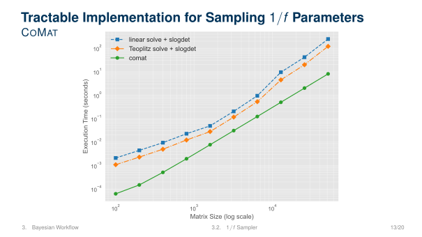
Tractable Implementation for Sampling 1/f Parameters COMAT: An O(n2) implementation Ncorr =   ξ0 ξ1 ξ2 · · · ξn−1 ξ1 ξ0 ξ1 · · · ξn−2 ξ2 ξ1 ξ0 · · · ξn−3 ... ... ... . . . ... ξn−1 ξn−2 ξn−3 · · · ξ0   • Recursive Determinant det  A B C D   = det(A)det(D−CA−1B). • Levinson-Durbin Recursion • Perturbative Scenario (Λ + P)−1 ≃ Λ−1 − m−1∑ k =0 Λ−1P [ −PΛ−1]k Λ−1. ln[det(Λ + P)] ≈ m−1∑ k =0 (−1)k k + 1 Tr [( PΛ−1) k +1] + ln[det(Λ)] 3. Bayesian Workflow 3.2. 1/f Sampler 12/20
Tractable Implementation for Sampling 1/f Parameters COMAT 102 103 104 Matrix Size (log scale) 10 4 10 3 10 2 10 1 100 101 102 Execution Time (seconds) linear solve + slogdet Teoplitz solve + slogdet comat 3. Bayesian Workflow 3.2. 1/f Sampler 13/20
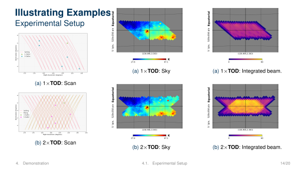
Illustrating Examples Experimental Setup 145150155160165170175 Right Ascension (degrees) 0 2 4 6 8Declination (degrees) Setting 1 CalSrc 5 CalSrc (a) 1×TOD: Scan 140145150155160165170175 Right Ascension (degrees) 0 2 4 6 8Declination (degrees) Setting Rising 1 CalSrc 5 CalSrc (b) 2×TOD: Scan 5 '/pix, 520x350 pixEquatorial (158.906,3.583) 27.8 67.1 K (a) 1×TOD: Sky 5 '/pix, 520x350 pixEquatorial (158.906,3.583) 27.8 67.1 K (b) 2×TOD: Sky 5 '/pix, 520x350 pixEquatorial (158.906,3.583) 0 60 (a) 1×TOD: Integrated beam. 5 '/pix, 520x350 pixEquatorial (158.906,3.583) 0 60 (b) 2×TOD: Integrated beam. 4. Demonstration 4.1. Experimental Setup 14/20
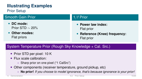
Illustrating Examples Prior Setup Smooth Gain Prior • DC mode: Prior STD ∼ 20% • Other modes: Flat priors 1/f Prior • Power law index: Flat prior • Reference (Knee) frequency: Flat prior System T emperature Prior (Rough Sky Knowledge + Cal. Src.) • Prior STD per pixel: 10 K • Flux scale calibration: ◦ Sharp prior on one pixel (“1 CalSrc”) • Other components (receiver temperature, ground pickup, etc) ◦ No prior! If you choose to model ignorance, that’s because ignorance is your prior! 4. Demonstration 4.2. Prior Setup 15/20
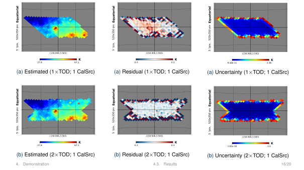
5 '/pix, 520x350 pixEquatorial (158.906,3.583) 27.8 67.1 K (a) Estimated (1×TOD; 1 CalSrc) 5 '/pix, 520x350 pixEquatorial (158.906,3.583) 27.8 67.1 K (b) Estimated (2×TOD; 1 CalSrc) 5 '/pix, 520x350 pixEquatorial (158.906,3.583) -0.3 0.3 K (a) Residual (1×TOD; 1 CalSrc) 5 '/pix, 520x350 pixEquatorial (158.906,3.583) -0.3 0.3 K (b) Residual (2×TOD; 1 CalSrc) 5 '/pix, 520x350 pixEquatorial (158.906,3.583) 9.44e-11 2.36 K (a) Uncertainty (1 ×TOD; 1 CalSrc) 5 '/pix, 520x350 pixEquatorial (158.906,3.583) 1.01e-10 2.5 K (b) Uncertainty (2 ×TOD; 1 CalSrc) 4. Demonstration 4.3. Results 16/20
An illustrating Example Histogram of the residuals across pixels 1.5 1.0 0.5 0.0 0.5 1.0 1.5 Tresidual = Tsample sky Ttrue sky [K] 0 5 10 15 20 25Probability Density 16th 84th pct = [-0.13, 0.17] K Figure: 1×TOD; 1 CalSrc 1.5 1.0 0.5 0.0 0.5 1.0 1.5 Tresidual = Tsample sky Ttrue sky [K] 0 10 20 30 40Probability Density 16th 84th pct = [-0.10, 0.03] K Figure: 2×TOD; 1 CalSrc 4. Demonstration 4.3. Results 17/20
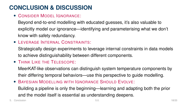
CONCLUSION & DISCUSSION • CONSIDER MODEL IGNORANCE : Beyond end-to-end modelling with educated guesses, it’s also valuable to explicitly model our ignorance—identifying and parameterising what we don’t know with safety redundancy . • LEVERAGE INTERNAL CONSTRAINTS : Strategically design experiments to leverage internal constraints in data models to achieve distinguishability between different components. • THINK LIKE THE TELESCOPE : MeerKA T -like observations can distinguish system temperature components by their differing temporal behaviors—use this perspective to guide modelling. • BAYESIAN MODELLING WITH IGNORANCE SHOULD EVOLVE : Building a pipeline is only the beginning—learning and adapting both the prior and the model itself is essential as understanding deepens. 5. Conclusion 5.0. 18/20
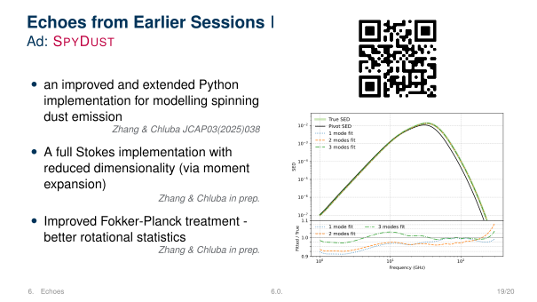
Echoes from Earlier Sessions I Ad: SPYDUST • an improved and extended Python implementation for modelling spinning dust emission Zhang & Chluba JCAP03(2025)038 • A full Stokes implementation with reduced dimensionality (via moment expansion) Zhang & Chluba in prep. • Improved Fokker-Planck treatment - better rotational statistics Zhang & Chluba in prep. 10 7 10 6 10 5 10 4 10 3 10 2 SED True SED Pivot SED 1 mode fit 2 modes fit 3 modes fit 100 101 102 Frequency (GHz) 0.9 1.0 1.1Fitted / True 1 mode fit 2 modes fit 3 modes fit 6. Echoes 6.0. 19/20
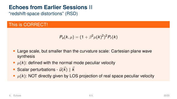
Echoes from Earlier Sessions II “redshift-space distortions” (RSD) This is CORRECT! Ps(k , µ) = ( 1 + β2µ(k )2)2Pr (k ) • Large scale, but smaller than the curvature scale: Cartesian plane wave synthesis • µ(k ): defined with the normal mode peculiar velocity • Scalar perturbations - ⃗u(⃗k ) ∥ ⃗k • µ(k ): NOT directly given by LOS projection of real space peculiar velocity 6. Echoes 6.0. 20/20