Modelling Spinning Dust Emissions

OUTLINE 1. Introduction 1.1. Spinning Dust Emission from the AME Perspective 1.2. Modelling Methodologies and Challenges 2. Our Efforts (on the Shoulders of Giants) 2.1. SpyDust: An Improved and Extended Implementation 2.2. A Perturbative Representation via Moment Expansion 2.3. On the rotation statistics 3. Conclusion

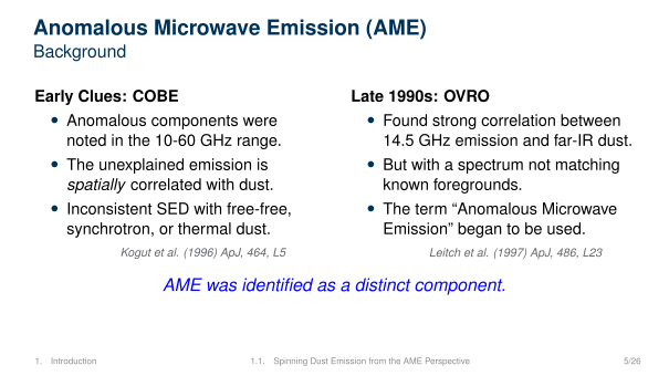
Anomalous Microwave Emission (AME) Background Early Clues: COBE • Anomalous components were noted in the 10-60 GHz range. • Inconsistent SED with free-free, synchrotron, or thermal dust. • But spatially correlated with dust. Kogut et al. (1996) ApJ, 464, L5 1. Introduction 1.1. Spinning Dust Emission from the AME Perspective 3/26

Anomalous Microwave Emission (AME) Background Late 1990s: OVRO • Found strong correlation between 14.5 GHz emission and far-IR dust. • But with a spectrum not matching known foregrounds. • The term “Anomalous Microwave Emission” began to be used. Leitch et al. (1997) ApJ, 486, L23 1. Introduction 1.1. Spinning Dust Emission from the AME Perspective 4/26

Anomalous Microwave Emission (AME) Background Early Clues: COBE • Anomalous components were noted in the 10-60 GHz range. • The unexplained emission is spatially correlated with dust. • Inconsistent SED with free-free, synchrotron, or thermal dust. Kogut et al. (1996) ApJ, 464, L5 Late 1990s: OVRO • Found strong correlation between 14.5 GHz emission and far-IR dust. • But with a spectrum not matching known foregrounds. • The term “Anomalous Microwave Emission” began to be used. Leitch et al. (1997) ApJ, 486, L23 AME was identiﬁed as a distinct component. 1. Introduction 1.1. Spinning Dust Emission from the AME Perspective 5/26

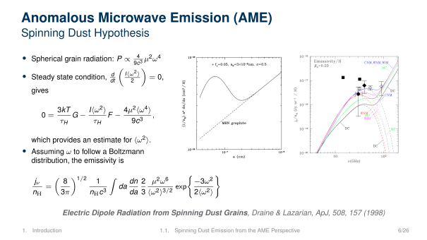
Anomalous Microwave Emission (AME) Spinning Dust Hypothesis • Spherical grain radiation: P ∝ 4 9c3 µ2ω4 • Steady state condition, d dt ( I⟨ω2⟩ 2 ) = 0, gives 0 = 3kT τH G − I⟨ω2⟩ τH F − 4µ2⟨ω4⟩ 9c3 , which provides an estimate for ⟨ω2⟩. • Assuming ω to follow a Boltzmann distribution, the emissivity is jν nH = ( 8 3π )1/2 1 nHc3 ∫ da dn da 2 3 µ2ω6 ⟨ω2⟩3/2 exp { −3ω2 2⟨ω2⟩ } Electric Dipole Radiation from Spinning Dust Grains , Draine & Lazarian, ApJ, 508, 157 (1998) 1. Introduction 1.1. Spinning Dust Emission from the AME Perspective 6/26

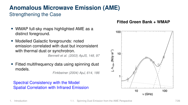
Anomalous Microwave Emission (AME) Strengthening the Case • WMAP full-sky maps highlighted AME as a distinct foreground. • Modelled Galactic foregrounds: noted emission correlated with dust but inconsistent with thermal dust or synchrotron. Bennett et al. (2003) ApJS, 148, 97 • Fitted multifrequency data using spinning dust models. Finkbeiner (2004) ApJ, 614, 186 Spectral Consistency with the Model Spatial Correlation with Infrared Emission Fitted Green Bank + WMAP 1. Introduction 1.1. Spinning Dust Emission from the AME Perspective 7/26

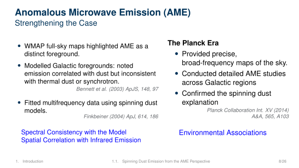
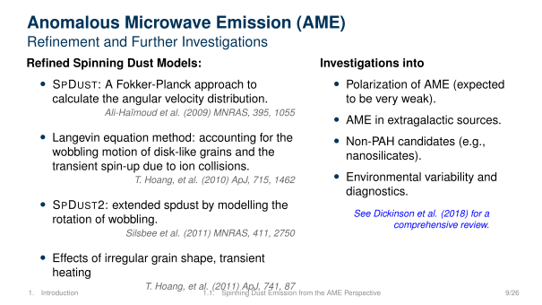
Anomalous Microwave Emission (AME) Reﬁnement and Further Investigations Reﬁned Spinning Dust Models: • SPDUST : A Fokker-Planck approach to calculate the angular velocity distribution. Ali-Haïmoud et al. (2009) MNRAS, 395, 1055 • Langevin equation method: accounting for the wobbling motion of disk-like grains and the transient spin-up due to ion collisions. T . Hoang, et al. (2010) ApJ, 715, 1462 • SPDUST 2: extended spdust by modelling the rotation of wobbling. Silsbee et al. (2011) MNRAS, 411, 2750 • Effects of irregular grain shape, transient heating T . Hoang, et al. (2011) ApJ, 741, 87 Investigations into • Polarization of AME (expected to be very weak). • AME in extragalactic sources. • Non-P AH candidates (e.g., nanosilicates). • Environmental variability and diagnostics. See Dickinson et al. (2018) for a comprehensive review. 1. Introduction 1.1. Spinning Dust Emission from the AME Perspective 9/26

Spinning Dust Emissions What’s left to uncover? 1. Introduction 1.2. Modelling Methodologies and Challenges 10/26

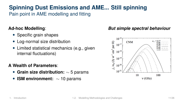
Spinning Dust Emissions and AME... Still spinning Pain point in AME modelling and ﬁtting Ad-hoc Modelling: • Speciﬁc grain shapes • Log-normal size distribution • Limited statistical mechanics (e.g., given internal ﬂuctuations) A Wealth of Parameters : • Grain size distribution: ∼ 5 params • ISM environment: ∼ 10 params But simple spectral behaviour 1. Introduction 1.2. Modelling Methodologies and Challenges 11/26

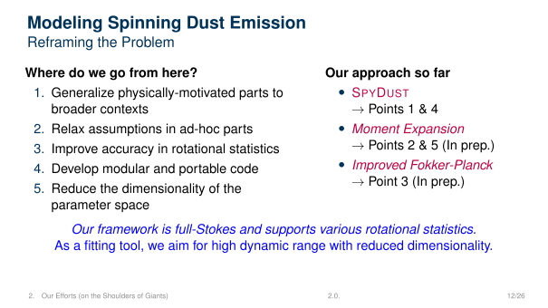
Modeling Spinning Dust Emission Reframing the Problem Where do we go from here? 1. Generalize physically-motivated parts to broader contexts 2. Relax assumptions in ad-hoc parts 3. Improve accuracy in rotational statistics 4. Develop modular and portable code 5. Reduce the dimensionality of the parameter space Our approach so far • SPYDUST → Points 1 & 4 • Moment Expansion → Points 2 & 5 (In prep.) • Improved Fokker-Planck → Point 3 (In prep.) Our framework is full-Stokes and supports various rotational statistics. As a ﬁtting tool, we aim for high dynamic range with reduced dimensionality . 2. Our Efforts (on the Shoulders of Giants) 2.0. 12/26

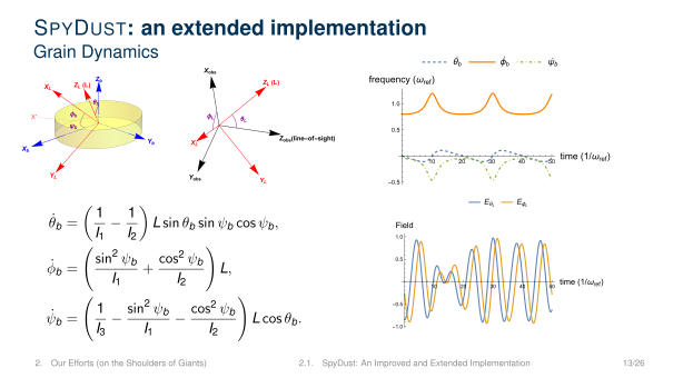
SPYDUST : an extended implementation Grain Dynamics ˙θb = 1 I1 − 1 I2 L sin θb sin ψb cos ψb, ˙ϕb = sin2 ψb I1 + cos2 ψb I2 ! L, ˙ψb = 1 I3 − sin2 ψb I1 − cos2 ψb I2 ! L cos θb. θb  ϕb  ψb  10 20 30 40 50 time(1/ω ref) -0.5 0.5 1.0 frequency(ω ref) EθL EϕL 10 20 30 40 50 time(1/ω ref) -1.0 -0.5 0.5 1.0 Field 2. Our Efforts (on the Shoulders of Giants) 2.1. SpyDust: An Improved and Extended Implementation 13/26

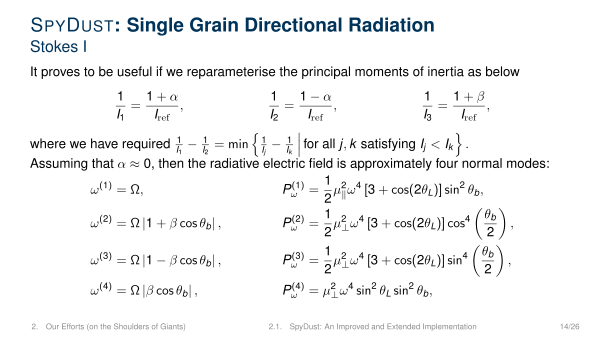
SPYDUST : Single Grain Directional Radiation Stokes I It proves to be useful if we reparameterise the principal moments of inertia as below 1 I1 = 1 + α Iref , 1 I2 = 1 − α Iref , 1 I3 = 1 + β Iref , where we have required 1 I1 − 1 I2 = min n 1 Ij − 1 Ik for all j, k satisfying Ij < Ik o . Assuming that α ≈ 0, then the radiative electric ﬁeld is approximately four normal modes: ω(1) = Ω, P(1) ω = 1 2 µ2 ∥ω4 [3 + cos(2θL)] sin2 θb, ω(2) = Ω |1 + β cos θb| , P(2) ω = 1 2 µ2 ⊥ω4 [3 + cos(2θL)] cos4 θb 2 , ω(3) = Ω |1 − β cos θb| , P(3) ω = 1 2 µ2 ⊥ω4 [3 + cos(2θL)] sin4 θb 2 , ω(4) = Ω |β cos θb| , P(4) ω = µ2 ⊥ω4 sin2 θL sin2 θb, 2. Our Efforts (on the Shoulders of Giants) 2.1. SpyDust: An Improved and Extended Implementation 14/26

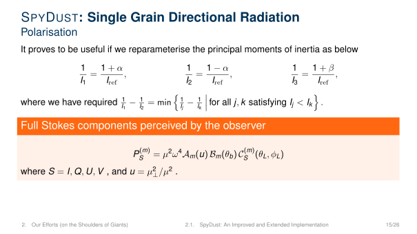
SPYDUST : Single Grain Directional Radiation Polarisation It proves to be useful if we reparameterise the principal moments of inertia as below 1 I1 = 1 + α Iref , 1 I2 = 1 − α Iref , 1 I3 = 1 + β Iref , where we have required 1 I1 − 1 I2 = min n 1 Ij − 1 Ik for all j, k satisfying Ij < Ik o . Full Stokes components perceived by the observer P(m) S = µ2ω4Am(u) Bm(θb) C(m) S (θL, ϕL) where S = I, Q, U, V , and u = µ2 ⊥/µ2 . 2. Our Efforts (on the Shoulders of Giants) 2.1. SpyDust: An Improved and Extended Implementation 15/26

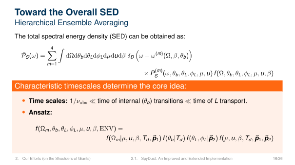
Toward the Overall SED Hierarchical Ensemble Averaging The total spectral energy density (SED) can be obtained as: ¯PS(ω) = 4X m=1 Z dΩdθbdθLdϕLdµdudβ δ D ω − ω(m)(Ω, β, θb) × P(m) S (ω, θb, θL, ϕL, µ, u) f (Ω, θb, θL, ϕL, µ, u, β) Characteristic timescales determine the core idea: • Time scales: 1/νobs ≪ time of internal ( θb) transitions ≪ time of L transport. • Ansatz: f (Ωm, θb, θL, ϕL, µ, u, β, ENV) = f (Ωm|µ, u, β, Td , ⃗p1) f (θb|Td ) f (θL, ϕL|⃗p2) f (µ, u, β, Td , ⃗p1, ⃗p2) 2. Our Efforts (on the Shoulders of Giants) 2.1. SpyDust: An Improved and Extended Implementation 16/26

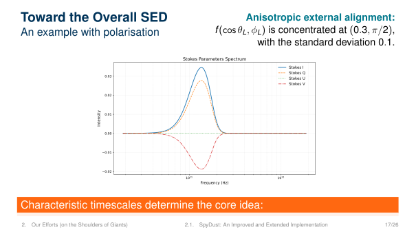
Toward the Overall SED An example with polarisation Anisotropic external alignment: f (cos θL, ϕL) is concentrated at (0.3, π/2), with the standard deviation 0 .1. 1011 1012 Frequency (Hz) 0.02 0.01 0.00 0.01 0.02 0.03 Intensity Stokes Parameters Spectrum Stokes I Stokes Q Stokes U Stokes V Characteristic timescales determine the core idea: 2. Our Efforts (on the Shoulders of Giants) 2.1. SpyDust: An Improved and Extended Implementation 17/26

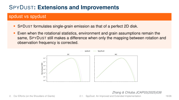
SPYDUST : Extensions and Improvements 100 101 102 [GHz] 10 20 10 15 10 10 10 5 100 Normalised SED a = 5 × 10 8 cm (disc-like) = -0.45 = -0.35 = -0.25 = -0.15 100 101 102 [GHz] 10 20 10 15 10 10 10 5 100 Normalised SED a = 5 × 10 7 cm (ellipsoidal) = -0.2 = 0.1 = 0 = 0.5 Zhang & Chluba JCAP03(2025)038 2. Our Efforts (on the Shoulders of Giants) 2.1. SpyDust: An Improved and Extended Implementation 18/26

SPYDUST : Extensions and Improvements spdust vs spydust • SPDUST formulates single-grain emission as that of a perfect 2D disk. • Even when the rotational statistics, environment and grain assumptions remain the same, S PYDUST still makes a difference when only the mapping between rotation and observation frequency is corrected. Zhang & Chluba JCAP03(2025)038 2. Our Efforts (on the Shoulders of Giants) 2.1. SpyDust: An Improved and Extended Implementation 19/26

Perturbative Representation with Derivative Spectra Formalism of moment expansion Abstractly , the total emission can be written in the following form: ¯PS(ν) = Z dp PS(ν, p)f (p), where p represents the parameter vector and PS denotes the integrand with the distribution f (p) factored out. T aylor expandingPS with respect to p around a pivot value ¯p: ¯PS(ν) = ∞X n1=0 · · · ∞X ns=0 W[n1,...,ns]Qs i=1 ni ! Θ[n1,...,ns](ν). where W[n1,...,ns] ≡ ⟨(p1 − ¯p1)n1 . . . (ps − ¯ps)ns ⟩, Θ[n1,...,ns] ≡ ∂n1 p1 . . . ∂ns ps PS ¯p. 2. Our Efforts (on the Shoulders of Giants) 2.2. A Perturbative Representation via Moment Expansion 20/26

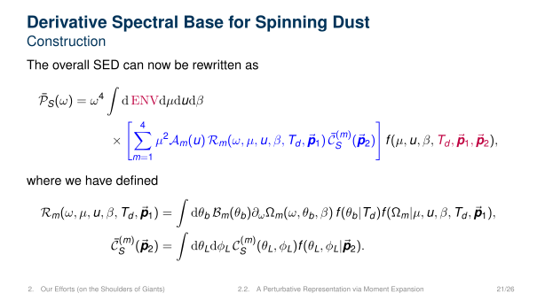
Derivative Spectral Base for Spinning Dust Construction The overall SED can now be rewritten as ¯PS(ω) = ω4 Z d ENVdµdudβ × " 4X m=1 µ2Am(u) Rm(ω, µ, u, β, Td , ⃗p1) ¯C(m) S (⃗p2) # f (µ, u, β, Td , ⃗p1, ⃗p2), where we have deﬁned Rm(ω, µ, u, β, Td , ⃗p1) = Z dθb Bm(θb)∂ωΩm(ω, θb, β) f (θb|Td )f (Ωm|µ, u, β, Td , ⃗p1), ¯C(m) S (⃗p2) = Z dθLdϕL C(m) S (θL, ϕL)f (θL, ϕL|⃗p2). 2. Our Efforts (on the Shoulders of Giants) 2.2. A Perturbative Representation via Moment Expansion 21/26

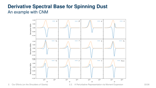
Derivative Spectral Base for Spinning Dust An example with CNM 0.10 0.05 0.00 0.05 0.10 Derivative SEDs a u 0.15 0.10 0.05 0.00 0.05 0.10 Derivative SEDs nh T xH 1011 1012 0.15 0.10 0.05 0.00 0.05 0.10 Derivative SEDs xC 1011 1012 y 1011 1012 1011 1012 atom 2. Our Efforts (on the Shoulders of Giants) 2.2. A Perturbative Representation via Moment Expansion 22/26

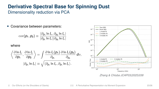
Derivative Spectral Base for Spinning Dust Dimensionality reduction via PCA • Covariance between parameters: cov(p1, p2) ≡ ⟨∂p1 ln Iν, ∂p2 ln Iν⟩ |∂p1 ln Iν||∂p2 ln Iν| where ∂ ln Iν ∂p1 , ∂ ln Iν ∂p2 = Z ∂ ln Iν(p1) ∂p1 ∂ ln Iν(p2) ∂p2 dν, |∂p1 ln Iν| ≡ q ⟨∂p1 ln Iν, ∂p1 ln Iν⟩. 10 7 10 6 10 5 10 4 10 3 10 2 SED True SED Pivot SED 1 mode fit 2 modes fit 3 modes fit 100 101 102 Frequency (GHz) 0.9 1.0 1.1Fitted / True 1 mode fit 2 modes fit 3 modes fit Zhang & Chluba JCAP03(2025)038 2. Our Efforts (on the Shoulders of Giants) 2.2. A Perturbative Representation via Moment Expansion 23/26

Rotation Statistics: Diffusion Approximation ∂t P(x, t) = R [w(x|x ′)P(x ′, t) − w(x ′|x)P(x, t)] dx ′ =⇒ ∂t P(x, t) =P∞ n=1 (−1)n n! ∂n ∂x n (an(x)P(x, t)), where an = R ξnw(x + ξ|x) dξ. T runcating at Second Order • Fokker–Planck Equation: ∂t P(x, t) = − ∂x [A(x)P(x, t)] + 1 2 ∂2 x [B(x)P(x, t)] • Applications ◦ A, B ⇒ P ◦ A, P ⇒ B ◦ B, P ⇒ A Figure: Solution to a 1D Fokker-Planck equation. 2. Our Efforts (on the Shoulders of Giants) 2.3. On the rotation statistics 24/26

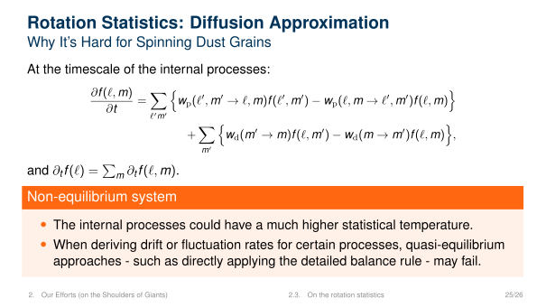
Rotation Statistics: Diffusion Approximation Why It’s Hard for Spinning Dust Grains At the timescale of the internal processes: ∂f (ℓ, m) ∂t = X ℓ′m′ n wp(ℓ′, m′ → ℓ, m)f (ℓ′, m′) − wp(ℓ, m → ℓ′, m′)f (ℓ, m) o + X m′ n wd(m′ → m)f (ℓ, m′) − wd(m → m′)f (ℓ, m) o , and ∂t f (ℓ) =P m ∂t f (ℓ, m). Non-equilibrium system • The internal processes could have a much higher statistical temperature. • When deriving drift or ﬂuctuation rates for certain processes, quasi-equilibrium approaches - such as directly applying the detailed balance rule - may fail. 2. Our Efforts (on the Shoulders of Giants) 2.3. On the rotation statistics 25/26

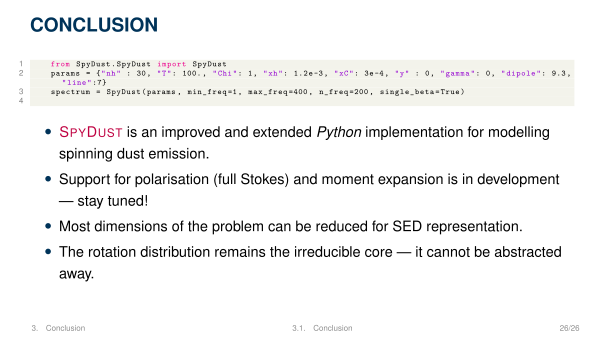
$CONCLUSION 1 from SpyDust . SpyDust import SpyDust 2 params = { " nh " : 30 , " T " : 100. , " Chi " : 1 , " xh " : 1.2 e -3 , " xC " : 3e -4 , " y " : 0 , " gamma " : 0 , " dipole " : 9.3 , " line " :7} 3 spe ct ru m = SpyDust ( params , m in_ fr eq =1 , m ax _f re q =400 , n_freq =200 , s i n g l e _ b e t a = True ) 4 • SPYDUST is an improved and extended Python implementation for modelling spinning dust emission. • Support for polarisation (full Stokes) and moment expansion is in development — stay tuned! • Most dimensions of the problem can be reduced for SED representation. • The rotation distribution remains the irreducible core — it cannot be abstracted away . 3. Conclusion 3.1. Conclusion 26/26$