Example 03 · Hierarchical inference notebook

Infer a population mean and eight group means from repeated noisy measurements. Follow the generative model, simulated observations and posterior estimates from the inference notebook.

Model and conditional structure

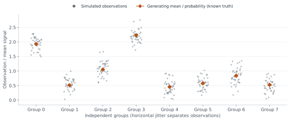
The population mean μ is shared. Each group has a latent mean u_g; its 40 observations share that mean. Known standard deviations are 0.6 between groups and 0.25 within a group.

\begin{aligned}\mu&\sim\operatorname{Uniform}(-3,3),\\u_g\mid\mu&\sim\mathcal N(\mu,0.6^2)\end{aligned}

y_{gj}\mid u_g\sim\mathcal N(u_g,0.25^2)

p(\mu,\mathbf u,\mathbf y)=p(\mu)\prod_{g=1}^{8}p(u_g\mid\mu)\prod_{j=1}^{40}p(y_{gj}\mid u_g)

This implementation uses a vector latent and an indexing operator. The fixed indices assign observations to groups.

Graph declaration

notebook_model.py

"""The hierarchical notebook's model. Run with: JAX_ENABLE_X64=1 python notebook_model.py"""

import jax.numpy as jnp
import numpy as np
import numpyro.distributions as dist

import bayesmith as bs

INDICES = np.repeat(np.arange(8), 40)
# Placeholder observations: the routes in the plan do not depend on their values.
DATA = jnp.asarray(np.random.default_rng(0).normal(size=INDICES.size))


def model(indices, data):
    """As recorded in the notebook run."""
    index = bs.const("group_index", indices)
    population = bs.sample("population", lambda: dist.Uniform(-3.0, 3.0))
    groups = bs.sample(
        "groups",
        lambda mu: dist.Normal(mu, 0.6).expand((8,)).to_event(1),
        population,
    )
    location = bs.det(
        "location", lambda u, i: u[i], groups, index, linear_in=("groups",)
    )
    bs.observe("obs", lambda loc: dist.Normal(loc, 0.25), location, obs=data)


if __name__ == "__main__":
    print(bs.compile(bs.trace(model, INDICES, DATA)))

Download this example

This restates the recorded model. The full example also constructs truths, simulates data and runs inference.

From simulated observations to inferred signal

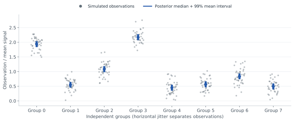
For this dataset, μ = 0.8. Group means were drawn from their conditional prior; observations were then simulated at those realized values. Switching views adds the inferred mean signal to the same measurements.

320 noisy measurements around eight realized group means — Gray points are observations; the orange diamonds mark the realized signal.

Posterior medians and 99 percent intervals for group means over simulated measurements — Blue points show the posterior median of each group mean; vertical intervals contain 99% posterior probability. This interval describes the group mean, not a future noisy observation.

Infer

The recorded run sampled both latents with NumPyro NUTS. This release compiles the same declaration to exact group means inside NUTS:

Block	Latents	Route	Why
0	`groups`	GCR exact	structurally certified; numerical check 3 scales x 3 at-points (max 0.00e+00)
1	`population`	NUTS	outside the exact block ['groups']: sampled by NUTS, and the exact block is solved CONDITIONAL on them, once per sweep
Execution		`HMCGibbs(inner=NUTS, gibbs_sites=['groups']); noise_std rebuilt every sweep`

Printed plan

block 0  {groups}         GCR exact         structurally certified; numerical check 3 scales x 3 at-points (max 0.00e+00)
         kappa=231.4 -> tol=4.3215212e-06, guard hoisted out of the sweep
         exact block ['groups']: sigma does not move with the block (0.000e+00 relative,
         rtol=1.0e-08), so the covariance is fixed and one Wiener solve is exact; the
         linearity check held ['population'] at their prior centre rather than drawing
         them -- they are not Gaussian, so their prior has no draw this module will
         take; the kappa sweep held ['population'] at their prior centre rather than
         moving them -- they are not Gaussian, so this module has no prior width to
         sweep them by, and the interval is not an interval in them
block 1  {population}     NUTS
         outside the exact block ['groups']: sampled by NUTS, and the exact block is
         solved CONDITIONAL on them, once per sweep
execution: HMCGibbs(inner=NUTS, gibbs_sites=['groups']); noise_std rebuilt every sweep

Recorded 2026-09-19 with bayesmith 0.9.0 on arm64 (accelerate BLAS, x64 on) from notebook_model.py. Condition numbers and tolerances in the printout depend on the BLAS; block membership and routes are re-checked by the test suite. Full record.

Given the population mean, the eight group means have a Gaussian prior (written with .expand, which only broadcasts one Normal to eight independent copies), each prediction selects one of them and the noise is fixed. The population mean has a uniform prior and is an ancestor of the group prior, so NUTS moves it. The plan was compiled on placeholder observations; the routes do not depend on the observed values. The figures below come from the recorded all-NUTS run.

Population and group recovery

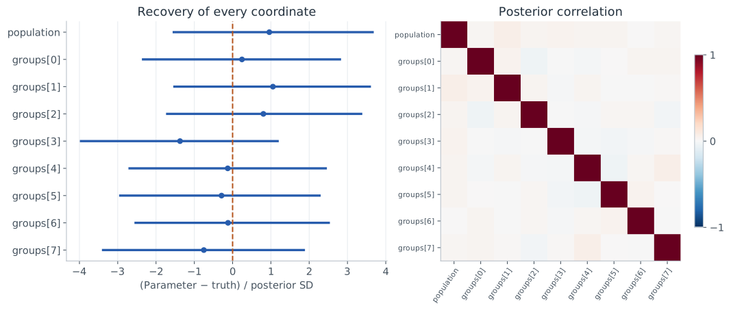
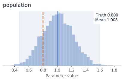
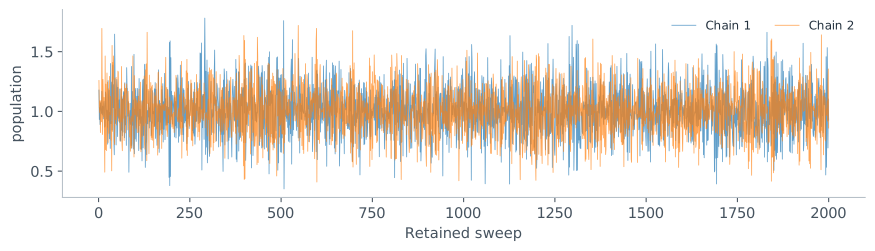
Repeated measurements constrain each group mean tightly. The population mean remains less precise because only eight groups inform it. Its posterior mean is 1.008 with standard deviation 0.217; the 99% interval is [0.467, 1.592], containing the generating value 0.8.

Posterior means and 99 percent intervals compared with the nine generating parameter values — Recovery is assessed against the realized group effects as well as the population value.

Marginal posterior distribution of the population mean with truth 0.8 — The population marginal retains uncertainty from variation between groups.

Chain diagnostics and provenance

The recorded NumPyro NUTS run retained 2,000 draws per chain after 1,000 warmup steps, with two chains and seed 0. It recorded zero divergences. Population R-hat was 1.000004. These diagnostics and the single-case recovery check do not establish simulation-based calibration.

Population chains and diagnostic values

Two retained MCMC chains for the population mean — Recorded population chains after warmup.

Quantity	Recorded value
Population ESS	8,817.25
Group-site ESS summary	7,251.43
Population R-hat	1.000004
Group-site R-hat summary	0.999925

ESS estimates are preserved as recorded and can exceed the retained draw count for negatively correlated draws. See diagnostic interpretation.

These figures are a historical notebook snapshot, associated with revision 6c644b1, rather than a new run of version 0.10.0. The downloadable record includes source hashes, model nodes, parameter summaries and figure checksums. Current runnable examples begin with Example 01 · First posterior.