Example 04 · Reweighting a Gaussian sample bank
When a prior is close to Gaussian but not Gaussian, the exact Gaussian route still supplies useful draws. Importance weights built from the full density ratio correct one bank of those draws to the non-Gaussian target, and the same bank serves every value of a population parameter. This two-cell example shows what changes at each step.
1. Define the population question
Let λ control the abundance of independent Poisson sources. Rescale their amplitudes so that the mean and variance stay fixed as λ changes. Higher-order structure then distinguishes populations that a covariance alone cannot separate.
Small λ
Rare, brighter sources.
More asymmetric fluctuations.
Large λ
Many, fainter sources.
Fluctuations approach a Gaussian.
Probability model for the illustration
Normal distributions here are parameterized by mean and variance. The two cells and diffuse Gaussian terms are independent conditional on λ. The prior field has mean zero and variance one for every λ; its third cumulant varies as
The observations are (0.5, −1.1). The full Poisson–Gaussian mixture density is evaluated; the teaching calculation truncates and renormalizes Poisson mass at a tail probability of 10−13. It does not use a truncated cumulant expansion.
2. Keep positions fixed; change their contribution
Each dot is a joint draw for both cells. The middle panel uses exactly the same positions as the left panel, colored by importance weight. The weighted marginal on the right can approximate the non-Gaussian posterior without moving the samples.
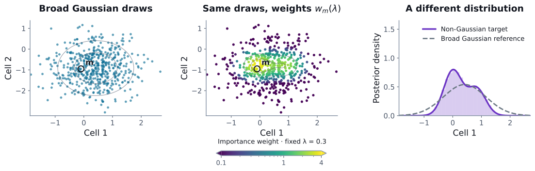
Scroll horizontally to compare panels, or open the full-size figure.
The proposal and the full density ratio
The reference q is a Gaussian proposal with standard deviation inflated by 1.8 relative to the conjugate Gaussian posterior. The plotted weights therefore include the likelihood, mixture prior and actual proposal density:
Z0 is a fixed Gaussian-model evidence, independent of λ. It rescales all weights equally. Normalized weights estimate posterior expectations; the average of unnormalized weights estimates Zλ/Z0. A prior-only ratio would be incorrect for this broadened proposal.
3. Vary the population parameter
Changing λ changes the weight of every draw. Positions, the circled draw and the logarithmic color scale stay fixed across the three panels, making the change in contribution directly comparable.
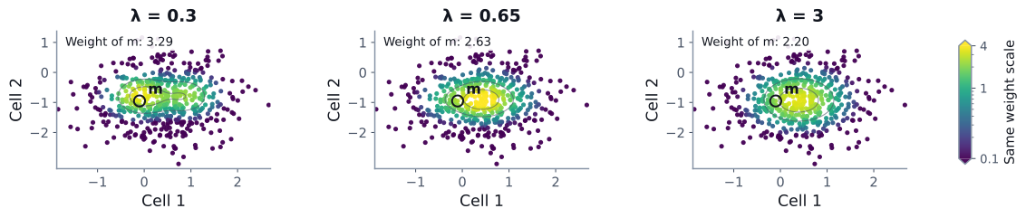
Scroll horizontally to compare panels, or open the full-size figure.
Average the unnormalized weights at each λ, include the hyperprior, then maximize the resulting marginal objective. The field variables have been integrated out by the sample average.

Scroll horizontally to compare panels, or open the full-size figure.
The recorded weighted MAP is 0.650; the analytic-convolution comparison gives 0.643. This agreement concerns this two-cell example and its fixed sample bank.
4. Separate sampling from repeated evaluation
Draw and retain the Gaussian bank.
Evaluate full density ratios and summarize the weights.
Check the fitted target with an independent bank or independent inference.
Reusing draws avoids paying the sampling cost for each candidate. Density evaluation, transformations and validation still contribute to total inference cost. The Gaussian draw timing in the seminar measures only the draw step and is not a benchmark for this full workflow.
Use the package interface
PosteriorReweighting implements fixed-reference-posterior recycling. Its graph constructor expects actual draws from the declared reference posterior; in the repository's inference example non_gaussian_reweight.py, that bank comes from the exact Gaussian route of a Gaussian reference graph. The broadened proposal q in these figures requires the full proposal-density ratio shown above; it must not be supplied as if it were that posterior.
Before applying recycling to a larger field, read the overlap and independent-bank requirements. A successful small example or a large ESS cannot rule out missed target mass.
Figure source and recorded validation
Adapted from the presentation sequence in seminar_talk_sep2026, pages 35–38. The original three figures and their numerical validation record are bundled unchanged. The provenance file records source and asset checksums. These historical teaching figures are separate from the current 0.10.0 release and from the seminar's large-field benchmark.