Example 06 · Prediction, simulation and checking
Continue from Example 05 using its recorded posterior and generated data. Generate a new observation, preserve its relationship to the posterior, then ask which discrepancies the model can reproduce.
Posterior prediction
The predictive section of five_tasks.py passes a posterior reference into PredictiveTask and the posterior object into execute_task. conditioned_sites names the observations defining the fit; replicated_sites requests newly generated observations; latent_sites selects retained latent draws.
An observed-data replay is not a replicated observation. Inspect replicated_draws for generated data and pointwise_log_density for scores. The latter carries an observation-unit/grouping contract: do not reinterpret correlated or vector events as independent measurements.
Compare generated observations
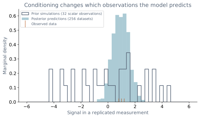
Scroll the figure horizontally, or open it for a full-size view.
SimulationResult and PredictiveResult outputs from five_tasks.py, seed 7: 32 scalar prior observations and 256 posterior predictive datasets of three measurements. Prior simulation follows the scalar Normal declared in the model; posterior replication retains the observed shape (256, 3). These are marginal histograms; measurements sharing a latent draw are correlated. The small prior simulation is deliberately coarse.The prior simulation asks what the model generates before seeing the data. The posterior prediction conditions on the three measurements and includes fresh observation noise.
Choose the source of parameters
| Parameter source | Meaning |
|---|---|
PRIOR | Sample the model's declared priors, then simulate downstream observations. |
FIXED | Supply named fixed values and generate observations at those settings. |
POSTERIOR_RESULT | Use the referenced posterior, checked against its conditioning and model fingerprints. |
Prior simulation samples each distribution the graph declares. Fixed and posterior-sourced simulation reuse the current predictive primitives. Their supported domains therefore differ; successful prior simulation does not imply that posterior replication is supported.
Evaluate a finished posterior
import jax
from five_tasks import main
from bayesmith.evaluation import check_posterior
from bayesmith.artifacts import ComputeBudget

graph, model_ref, posterior, predictive, evidence = main()

gate = check_posterior(
    graph, posterior, key=jax.random.key(90),
    budget=ComputeBudget(draws=512), model_ref=model_ref,
)
This continuation uses the graph, model reference and posterior returned by five_tasks.main(). It requests the checks that apply, not a guaranteed PASS. Review each report's applicability, conclusion and grounds. Floors and optional inputs may produce an unverifiable report.
Read the recorded check
| Quantity | Recorded output |
|---|---|
| Operational status | evaluated |
| Verdict | pass |
| Diagnostic warning | Estimated shape parameter of Pareto distribution is greater than 0.58 for one or more samples. You should consider using a more robust model, this is because importance sampling is less likely to work well if the marginal posterior and LOO posterior are very different. This is more likely to happen with a non-robust model and highly influential observations. |
This is the actual outcome of the continuation above with key 90. A verdict applies to the required checks on this posterior; it does not certify every optional check or establish calibration. The recorded PSIS warning is retained even though the required checks pass: the LOO estimate needs separate attention. Missing diagnostics remain missing. See the shared run record for the data and environment.
Current predictive boundary
Replicated prediction currently admits diagonal-Gaussian observed nodes. Correlated or non-Gaussian observation laws are refused as predictive_noise_unsupported; posterior inference may still be available on the same graph.
See diagnostics and model checks for the interpretation of PASS, FAIL and ABSTAIN.