Example 05 · Five questions, one model
After Example 01, keep the same simple model and ask five different statistical questions. Use an explicit task when the question, budget and provenance must travel with the answer.
Pick the statistical quantity first
| Question | Task → Result |
|---|---|
| What remains uncertain about the parameters? | PosteriorTask → PosteriorResult |
| Which point summary do I want? | PointEstimateTask → PointEstimateResult |
| What observations could this posterior predict? | PredictiveTask → PredictiveResult |
| What does the forward model generate? | SimulationTask → SimulationResult |
| What is the normalized probability of these data? | EvidenceTask → EvidenceResult |
Compilation and execution can return Refusal. Check both boundaries before consuming the result. A numerical execution failure can raise an exception; it is not a statistical conclusion about the model.
Run the complete workflow
Save the script as a file so the model source can be fingerprinted. Run JAX_ENABLE_X64=1 python five_tasks.py. Each successful stage prints its Result type; the final round trip checks artifact identity.
Complete runnable script
"""Run with JAX_ENABLE_X64=1 python five_tasks.py."""

from pathlib import Path
from tempfile import TemporaryDirectory

import jax
import jax.numpy as jnp
import numpyro.distributions as dist

import bayesmith as bs
from bayesmith.artifacts import (
    ArtifactKind,
    ArtifactRef,
    ComputeBudget,
    Estimand,
    EvidenceResult,
    EvidenceTask,
    ParameterSource,
    ParameterSourceKind,
    PointEstimateResult,
    PointEstimateTask,
    PosteriorResult,
    PosteriorTask,
    PredictiveResult,
    PredictiveTask,
    Refusal,
    SimulationResult,
    SimulationTask,
    dump_artifact,
    load_artifact,
    model_ref_from_callable,
    new_task_meta,
)


def model(data):
    level = bs.sample("level", lambda: dist.Normal(0.0, 2.0))
    bs.observe("signal", lambda x: dist.Normal(x, 0.5), level, obs=data)


def run_workflow():
    """Return each result so the tutorial can plot what was actually run."""
    graph = bs.trace(model, jnp.array([0.8, 1.0, 1.2]))
    model_ref = model_ref_from_callable(model, identifier="level-example")
    keys = iter(jax.random.split(jax.random.key(7), 10))

    def run(task, expected, source=None):
        planned = bs.compile_task(graph, task, model_ref=model_ref, key=next(keys))
        if isinstance(planned, Refusal):
            raise SystemExit(planned.failed_premise)
        result = bs.execute_task(planned, key=next(keys), source_posterior=source)
        if isinstance(result, Refusal):
            raise SystemExit(result.failed_premise)
        assert isinstance(result, expected)
        print(type(result).__name__)
        return result

    # 1. Posterior: retain uncertainty about the latent level.
    posterior = run(
        PosteriorTask(
            meta=new_task_meta(label="level posterior"),
            budget=ComputeBudget(draws=256),
        ),
        PosteriorResult,
    )

    # 2. Point estimate: ask explicitly for the posterior mean.
    point = run(
        PointEstimateTask(
            meta=new_task_meta(label="level mean"),
            estimand=Estimand.POSTERIOR_MEAN,
        ),
        PointEstimateResult,
    )
    print({array.name: array.value for array in point.values})

    # 3. Predictive: replicate the measurements using this posterior.
    source_ref = ArtifactRef(
        artifact_id=posterior.meta.artifact_id,
        revision=posterior.meta.revision,
        artifact_type=ArtifactKind.RESULT,
    )
    predictive = run(
        PredictiveTask(
            meta=new_task_meta(label="replicate signal"),
            source_posterior_ref=source_ref,
            conditioned_sites=("signal",),
            replicated_sites=("signal",),
            latent_sites=("level",),
        ),
        PredictiveResult,
        source=posterior,
    )
    print(predictive.replicated_draws[0].value.shape)

    # 4. Simulation: sample from the declared prior, then generate data.
    simulation = run(
        SimulationTask(
            meta=new_task_meta(label="prior simulation"),
            parameter_source=ParameterSource(kind=ParameterSourceKind.PRIOR),
            latent_sites=("level",),
            observed_sites=("signal",),
            budget=ComputeBudget(draws=32),
        ),
        SimulationResult,
    )

    # 5. Evidence: x64 and a fully normalized linear-Gaussian model.
    evidence = run(
        EvidenceTask(meta=new_task_meta(label="analytic evidence")), EvidenceResult
    )
    print("log p(data):", evidence.log_evidence)

    # Store data artifacts, never a live Graph or compiled executable.
    with TemporaryDirectory() as directory:
        path = Path(directory) / "posterior.json"
        dump_artifact(posterior, path)
        restored = load_artifact(path)
        assert isinstance(restored, PosteriorResult)
        assert restored.meta.artifact_id == posterior.meta.artifact_id
    print("Artifact round trip: identity preserved")
    return {
        "graph": graph,
        "model_ref": model_ref,
        "posterior": posterior,
        "point": point,
        "predictive": predictive,
        "simulation": simulation,
        "evidence": evidence,
    }


def main():
    results = run_workflow()
    return tuple(
        results[name]
        for name in ("graph", "model_ref", "posterior", "predictive", "evidence")
    )


if __name__ == "__main__":
    main()
What the run returns
| Result | Recorded output |
|---|---|
| PosteriorResult | 256 level draws; mean 0.9633 |
| PointEstimateResult | Posterior mean 0.9796 |
| PredictiveResult | Replicated signal shape (256, 3) |
| SimulationResult | Prior simulation shape (32,) |
| EvidenceResult | log p(data) = -2.905733 |
| Artifact round trip | Identity preserved (asserted during execution) |
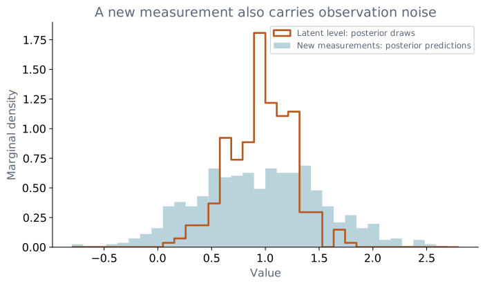
Scroll the figure horizontally, or open it for a full-size view.
The run record contains the numerical draws, captured console output, software versions, source hashes and figure checksums. This one-data-set example demonstrates the workflow, not calibration across datasets.
Understand the references
A predictive task stores a reference to its source posterior; execution receives the actual posterior separately. Results and provenance explains identity checks and reuse.
The point task requests POSTERIOR_MEAN. Changing it to MAP changes the estimand even when both coincide in this symmetric Gaussian example. The simulation task draws from the prior; it does not reuse the posterior unless you declare that parameter source.
Supported models
These five tasks work on this deliberately simple graph. General posterior sampling has wider support than replicated prediction, and whole-graph analytic evidence has stronger normalization and structure requirements than posterior sampling. A successful Gaussian tutorial does not certify arbitrary graphs.
Next: prediction and simulation, or results and provenance.